728x90
반응형
seaborn
- matplot 모듈 기능, 스타일 확장한 고급 시각화 도구, 데이터 셋 저장 모듈
import seaborn as sns
print(sns.get_dataset_names())
titanic = sns.load_dataset('titanic')
# ['anagrams', 'anscombe', 'attention', 'brain_networks', 'car_crashes', 'diamonds', 'dots', 'exercise', 'flights', 'fmri', 'gammas', 'geyser', 'iris', 'mpg', 'penguins', 'planets', 'tips', 'titanic']
print(titanic.head())
survived pclass sex age sibsp parch fare embarked class \
0 0 3 male 22.0 1 0 7.2500 S Third
1 1 1 female 38.0 1 0 71.2833 C First
2 1 3 female 26.0 0 0 7.9250 S Third
3 1 1 female 35.0 1 0 53.1000 S First
4 0 3 male 35.0 0 0 8.0500 S Third
who adult_male deck embark_town alive alone
0 man True NaN Southampton no False
1 woman False C Cherbourg yes False
2 woman False NaN Southampton yes True
3 woman False C Southampton yes False
4 man True NaN Southampton no Trueprint(titanic.info())
<class 'pandas.core.frame.DataFrame'>
RangeIndex: 891 entries, 0 to 890
Data columns (total 15 columns):
# Column Non-Null Count Dtype
--- ------ -------------- -----
0 survived 891 non-null int64
1 pclass 891 non-null int64
2 sex 891 non-null object
3 age 714 non-null float64
4 sibsp 891 non-null int64
5 parch 891 non-null int64
6 fare 891 non-null float64
7 embarked 889 non-null object
8 class 891 non-null category
9 who 891 non-null object
10 adult_male 891 non-null bool
11 deck 203 non-null category
12 embark_town 889 non-null object
13 alive 891 non-null object
14 alone 891 non-null bool
dtypes: bool(2), category(2), float64(2), int64(4), object(5)
memory usage: 80.6+ KB
Nonesns.set_style('darkgrid')
# darkgrid, whitegrid, dark, white, ticks 등
fig = plt.figure(figsize = (15, 5)) # fig 크기
ax1 = fig.add_subplot(1,2,1) # 위
ax2 = fig.add_subplot(1,2,2) # 아래
# 선형회귀, 산점도
sns.regplot(x='age',
y='fare',
data = titanic,
ax = ax1)
sns.regplot(x='age',
y='fare',
data = titanic,
ax = ax2,
fit_reg=False)
plt.show()
히스토그램
- distplot 두개 다
- kedplot 선형 분포
- histplot 막대 분포
fig = plt.figure(figsize = (15, 5)) # fig 크기
ax1 = fig.add_subplot(1,3,1) # 위
ax2 = fig.add_subplot(1,3,2) # 아래
ax3 = fig.add_subplot(1,3,3) # 아래
# distplot : 합친 것
sns.distplot(titanic['fare'], ax=ax1)
# kdeplot : 커널 밀도
sns.kdeplot(x='fare', data =titanic, ax=ax2)
# sns.distplot(titanic['fare'], hist = False, ax=ax1)
# histplot : 히스토그램
sns.histplot(x='fare', data =titanic, ax=ax3)
# sns.distplot(titanic['fare'], kde = False, ax=ax1)

ax1.set_title('titanic fare - distplot')
ax2.set_title('titanic fare - kdeplot')
ax3.set_title('titanic fare - histplot')
plt.show()
히트맵
sns.set_style('darkgrid')
# 피벗테이블로 범주현 변수를 각각 행, 열로 재구분하여 정리
table = titanic.pivot_table(index = ['sex'], columns = ['class'], aggfunc='size')
# 성별이 인덱스, 컬럼이 탑승등급, aggdfunc 건수 표시
# 피벗테이블 : 범위를 가지는 값 별로 건수로 출력되는 테이블
# 히트맵 그리기
sns.heatmap(table,                  # 데이터 프레임
           annot = True, fmt = 'd', # 데이터 값 표시, 정수형 포맷
           cmap='YlGnBu',           # 컬러맵
           linewidth=5,             # 구분선
           cbar=True)              # 컬러 바 표시 여부

plt.show()
# 산점도
sns.set_style('whitegrid')
fig = plt.figure(figsize = (15,5))
ax1 = fig.add_subplot(1,2,1) # 위
ax2 = fig.add_subplot(1,2,2) # 아래
# 이산형 변수 의 분포 데이터 분산 미고려
sns.stripplot(x = 'class',
            y = 'age',
            data = titanic,
            ax = ax1)
# 이산형 변수의 분포 : 데이터 분산 고려, 중복 없음, 겹치지 않게 옆으로 밀어냄
sns.swarmplot(x = 'class',
            y = 'age',
            data = titanic,
            ax = ax2)
# 차트제목 표시
ax1.set_title('Strip Plot')
ax2.set_title('Swarm Plot')
plt.show()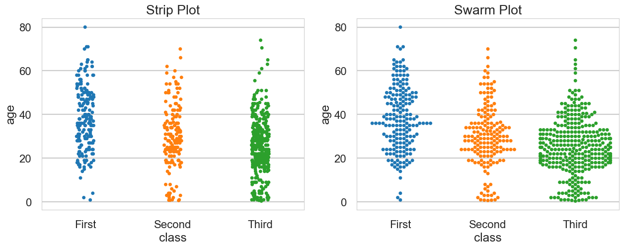
# 산점도
sns.set_style('whitegrid')
fig = plt.figure(figsize = (15,5))
ax1 = fig.add_subplot(1,2,1) # 위
ax2 = fig.add_subplot(1,2,2) # 아래
# 이산형 변수 의 분포 데이터 분산 미고려
sns.stripplot(x = 'class',
            y = 'age',
            data = titanic,
            hue = 'sex', # 데이터 구분 컬럼 // 동일 배치에 색깔로 구분
            ax = ax1)
# 이산형 변수의 분포 : 데이터 분산 고려, 중복 없음, 겹치지 않게 옆으로 밀어냄
sns.swarmplot(x = 'class',
            y = 'age',
            data = titanic,
            hue = 'sex',
            ax = ax2)
# 차트제목 표시
ax1.set_title('Strip Plot')
ax2.set_title('Swarm Plot')
ax1.legend(loc = 'upper right')
ax2.legend(loc = 'upper right')
plt.show()
# 막대 그래프
fig = plt.figure(figsize = (15,5))
ax1 = fig.add_subplot(1,3,1) # 위
ax2 = fig.add_subplot(1,3,2) # 아래
ax3 = fig.add_subplot(1,3,3) # 아래

sns.barplot(x='sex', y='survived', data=titanic, ax=ax1)
sns.barplot(x='sex', y='survived', hue = 'class', data=titanic, ax=ax2)
sns.barplot(x='sex', y='survived', hue = 'class', dodge = False, data=titanic, ax=ax3)

# 차트제목 표시
ax1.set_title('titanic survived  sex')
ax2.set_title('titanic survived  sex/class')
ax3.set_title('titanic survived  sex/class(stacked)')
plt.show()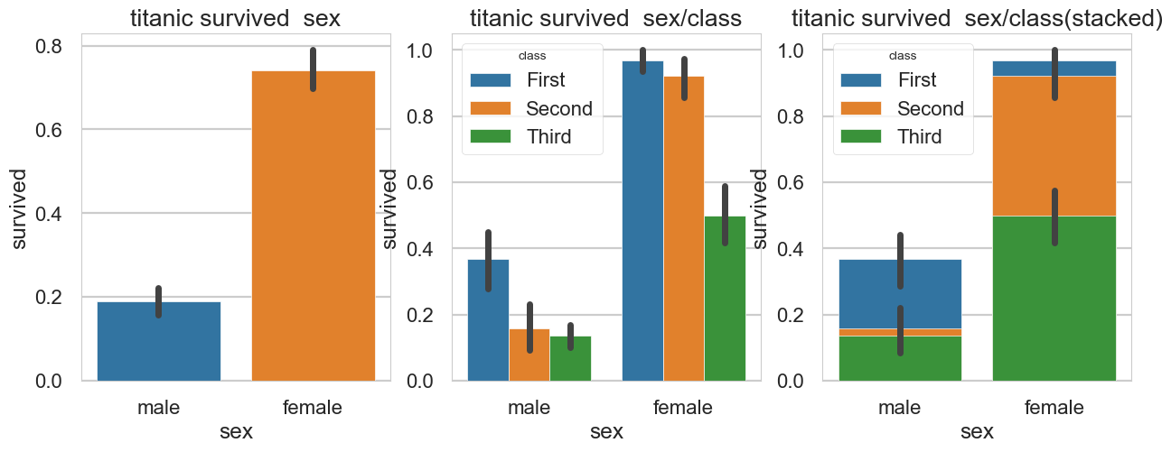
# countplot 막대 그래프 건수 출력
fig = plt.figure(figsize = (15,5))
ax1 = fig.add_subplot(1,3,1) # 위
ax2 = fig.add_subplot(1,3,2) # 아래
ax3 = fig.add_subplot(1,3,3) # 아래

sns.countplot(x='class', palette='Set1', data=titanic, ax=ax1)
sns.countplot(x='class', hue = 'who', palette='Set1', data=titanic, ax=ax2)
sns.countplot(x='class', hue = 'who', palette='Set1', dodge = False, data=titanic, ax=ax3)
# 차트제목 표시
ax1.set_title('titanic survived')
ax2.set_title('titanic survived - who')
ax3.set_title('titanic survived - who(stacked)')
plt.show()
# boxplot 막대 그래프 건수 출력
fig = plt.figure(figsize = (15,5))
ax1 = fig.add_subplot(2,2,1) # 위
ax2 = fig.add_subplot(2,2,2) # 아래
ax3 = fig.add_subplot(2,2,3) # 아래
ax4 = fig.add_subplot(2,2,4) # 아래

sns.boxplot(x='alive', y= 'age', data=titanic, ax=ax1)
sns.boxplot(x='alive', y= 'age', hue = 'sex', data=titanic, ax=ax2)
sns.violinplot(x='alive', y='age', data=titanic, ax=ax3)
sns.violinplot(x='alive', y='age', hue = 'sex', data=titanic, ax=ax4)

# 차트제목 표시
ax2.legend(loc='upper center')
ax4.legend(loc='upper center')
plt.show()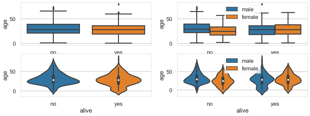
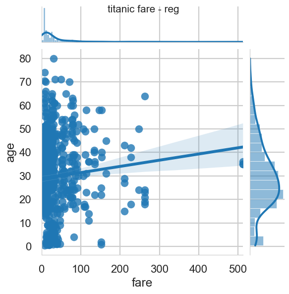
# 조인트그래프 - 산점도
j1 = sns.jointplot(x='fare', y= 'age', data=titanic)
# 조인트그래프 - 회귀선
j2 = sns.jointplot(x='fare', y= 'age', kind = 'reg', data=titanic)
# 조인트그래프 - 육각 그래프
j3 = sns.jointplot(x='fare', y='age', kind = 'hex', data=titanic)
# 조인트그래프 - 커럴 밀집 그래프
j4 = sns.jointplot(x='fare', y='age', kind = 'kde', data=titanic)

# 차트제목 표시
j1.fig.suptitle('titanic fare - scatter',size = 15)
j2.fig.suptitle('titanic fare - reg',size = 15)
j3.fig.suptitle('titanic fare - hex',size = 15)
j4.fig.suptitle('titanic fare - kde',size = 15)
plt.show()


# 조건에 따라 그리드 나누기
# who : man, woman, child
# survived : 0 1
g = sns.FacetGrid(data = titanic, col='who', row='survived') # 한방에, 컬럼 로우별
# 그래프 적용하기
g = g.map(plt.hist, 'age')
plt.show()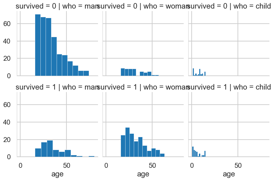
# 이변수 데이터 분포 그리기 pairplot
# 각변수들의 산점도 출력, 대각선 위치의 그래프는 히스토그램 으로 표시
# pairplot
titanic_pair = titanic[['age', 'pclass', 'fare']]
print(titanic_pair)
# 조건에 따라 그리드 나누기
g = sns.pairplot(titanic_pair)

      age  pclass     fare
0    22.0       3   7.2500
1    38.0       1  71.2833
2    26.0       3   7.9250
3    35.0       1  53.1000
4    35.0       3   8.0500
..    ...     ...      ...
886  27.0       2  13.0000
887  19.0       1  30.0000
888   NaN       3  23.4500
889  26.0       1  30.0000
890  32.0       3   7.7500

[891 rows x 3 columns]
반응형
'Data_Science > Data_Analysis_Py' 카테고리의 다른 글
| 8. iris || '21.06.28. (0) | 2021.10.26 |
|---|---|
| 7. folium || '21.06.24. (0) | 2021.10.26 |
| 5. auto-mpg 분석 || '21.06.24. (0) | 2021.10.26 |
| 4. 시도별 전출입 인구수 분석 ( 2 || '21.06.24. (0) | 2021.10.26 |
| 3. 시도별 전출입 인구수 분석 ( 1 || 2021.06.23 (0) | 2021.10.26 |