728x90
반응형
K-Means를 이용한 붓꽃(Iris) 데이터 셋 Clustering
centroid 기반, 가장많이 활용
from sklearn.datasets import load_iris
from sklearn.cluster import KMeans
import matplotlib.pyplot as plt
import numpy as np
import pandas as pd
%matplotlib inline

iris = load_iris()

# 보다 편리한 데이터 Handling을 위해 DataFrame으로 변환
irisDF = pd.DataFrame(data=iris.data, columns=['sepal_length','sepal_width','petal_length','petal_width'])
irisDF.head(3)

	sepal_length	sepal_width	petal_length	petal_width
0	5.1	3.5	1.4	0.2
1	4.9	3.0	1.4	0.2
2	4.7	3.2	1.3	0.2
KMeans 객체를 생성하고 군집화 수행
kmeans = KMeans(n_clusters=3, init='k-means++', max_iter=300,random_state=0)
kmeans.fit(irisDF)


KMeans(algorithm='auto', copy_x=True, init='k-means++', max_iter=300,
    n_clusters=3, n_init=10, n_jobs=1, precompute_distances='auto',
    random_state=0, tol=0.0001, verbose=0)
labels_ 속성을 통해 각 데이터 포인트별로 할당된 군집 중심점(Centroid)확인하고 irisDF에 'cluster' 컬럼으로 추가
print(kmeans.labels_)
print(kmeans.predict(irisDF))


[1 1 1 1 1 1 1 1 1 1 1 1 1 1 1 1 1 1 1 1 1 1 1 1 1 1 1 1 1 1 1 1 1 1 1 1 1
 1 1 1 1 1 1 1 1 1 1 1 1 1 0 0 2 0 0 0 0 0 0 0 0 0 0 0 0 0 0 0 0 0 0 0 0 0
 0 0 0 2 0 0 0 0 0 0 0 0 0 0 0 0 0 0 0 0 0 0 0 0 0 0 2 0 2 2 2 2 0 2 2 2 2
 2 2 0 0 2 2 2 2 0 2 0 2 0 2 2 0 0 2 2 2 2 2 0 2 2 2 2 0 2 2 2 0 2 2 2 0 2
 2 0]
irisDF['cluster']=kmeans.labels_
irisDF['target'] = iris.target
iris_result = irisDF.groupby(['target','cluster'])['sepal_length'].count()
print(iris_result)


target  cluster
0       1          50
1       0          48
        2           2
2       0          14
        2          36
Name: sepal_length, dtype: int64
iris.target_names

array(['setosa', 'versicolor', 'virginica'], dtype='<U10')
2차원 평면에 데이터 포인트별로 군집화된 결과를 나타내기 위해 2차원 PCA값으로 각 데이터 차원축소
from sklearn.decomposition import PCA

pca = PCA(n_components=2)
pca_transformed = pca.fit_transform(iris.data)

irisDF['pca_x'] = pca_transformed[:,0]
irisDF['pca_y'] = pca_transformed[:,1]
irisDF.head(3)


	sepal_length	sepal_width	petal_length	petal_width	cluster	target	pca_x	pca_y
0	5.1	3.5	1.4	0.2	1	0	-2.684207	0.326607
1	4.9	3.0	1.4	0.2	1	0	-2.715391	-0.169557
2	4.7	3.2	1.3	0.2	1	0	-2.889820	-0.137346
plt.scatter(x=irisDF.loc[:, 'pca_x'], y=irisDF.loc[:, 'pca_y'], c=irisDF['cluster'])
# cluster 값이 0, 1, 2 인 경우마다 별도의 Index로 추출
marker0_ind = irisDF[irisDF['cluster']==0].index
marker1_ind = irisDF[irisDF['cluster']==1].index
marker2_ind = irisDF[irisDF['cluster']==2].index

# cluster값 0, 1, 2에 해당하는 Index로 각 cluster 레벨의 pca_x, pca_y 값 추출. o, s, ^ 로 marker 표시
plt.scatter(x=irisDF.loc[marker0_ind,'pca_x'], y=irisDF.loc[marker0_ind,'pca_y'], marker='o')
plt.scatter(x=irisDF.loc[marker1_ind,'pca_x'], y=irisDF.loc[marker1_ind,'pca_y'], marker='s')
plt.scatter(x=irisDF.loc[marker2_ind,'pca_x'], y=irisDF.loc[marker2_ind,'pca_y'], marker='^')

plt.xlabel('PCA 1')
plt.ylabel('PCA 2')
plt.title('3 Clusters Visualization by 2 PCA Components')
plt.show()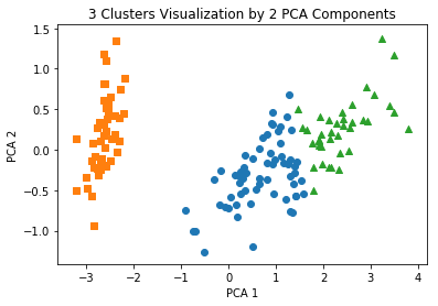
반응형
'Data_Science > ML_Perfect_Guide' 카테고리의 다른 글
| 7-3. Cluster_evaluation || 실루엣 계수 (0) | 2021.12.30 |
|---|---|
| 7-2. Kmeans 2 (0) | 2021.12.29 |
| 6-6. NMF (Non Negative Matrix Factorization) (0) | 2021.12.29 |
| 6-5. Truncated SVD (0) | 2021.12.29 |
| 6-4. SVD (singular value decomposition) (0) | 2021.12.29 |