728x90
반응형
기계학습 각각변수들의 관계를 찾는 과정
- 예측:회귀분석
- 분류:knn
- 군집:Kmeans
- 머신러닝 프로세스 -> 데이터 분리 -> 알고리즘 준비-> 모형학습 -> 예측 -> 평가 -> 활용
# 회귀분석 : 가격, 매출, 주가 등 연속성 데이터 예측 알고리즘 import pandas as pd import numpy as np import matplotlib.pyplot as plt import seaborn as sns df = pd.read_csv('auto-mpg.csv', header = None) df.columns = ['mpg', 'cylinders', 'displacement', 'horsepower','weight','acceleration', 'model year', 'origin', 'name'] df mpg cylinders displacement horsepower weight acceleration model year origin name 0 18.0 8 307.0 130.0 3504.0 12.0 70 1 chevrolet chevelle malibu 1 15.0 8 350.0 165.0 3693.0 11.5 70 1 buick skylark 320 2 18.0 8 318.0 150.0 3436.0 11.0 70 1 plymouth satellite 3 16.0 8 304.0 150.0 3433.0 12.0 70 1 amc rebel sst 4 17.0 8 302.0 140.0 3449.0 10.5 70 1 ford torino ... ... ... ... ... ... ... ... ... ... 393 27.0 4 140.0 86.00 2790.0 15.6 82 1 ford mustang gl 394 44.0 4 97.0 52.00 2130.0 24.6 82 2 vw pickup 395 32.0 4 135.0 84.00 2295.0 11.6 82 1 dodge rampage 396 28.0 4 120.0 79.00 2625.0 18.6 82 1 ford ranger 397 31.0 4 119.0 82.00 2720.0 19.4 82 1 chevy s-10 398 rows × 9 columns
print(df.info()) <class 'pandas.core.frame.DataFrame'> RangeIndex: 398 entries, 0 to 397 Data columns (total 9 columns): # Column Non-Null Count Dtype --- ------ -------------- ----- 0 mpg 398 non-null float64 1 cylinders 398 non-null int64 2 displacement 398 non-null float64 3 horsepower 398 non-null object 4 weight 398 non-null float64 5 acceleration 398 non-null float64 6 model year 398 non-null int64 7 origin 398 non-null int64 8 name 398 non-null object dtypes: float64(4), int64(3), object(2) memory usage: 28.1+ KB None
print(df.describe()) mpg cylinders displacement weight acceleration \ count 398.000000 398.000000 398.000000 398.000000 398.000000 mean 23.514573 5.454774 193.425879 2970.424623 15.568090 std 7.815984 1.701004 104.269838 846.841774 2.757689 min 9.000000 3.000000 68.000000 1613.000000 8.000000 25% 17.500000 4.000000 104.250000 2223.750000 13.825000 50% 23.000000 4.000000 148.500000 2803.500000 15.500000 75% 29.000000 8.000000 262.000000 3608.000000 17.175000 max 46.600000 8.000000 455.000000 5140.000000 24.800000 model year origin count 398.000000 398.000000 mean 76.010050 1.572864 std 3.697627 0.802055 min 70.000000 1.000000 25% 73.000000 1.000000 50% 76.000000 1.000000 75% 79.000000 2.000000 max 82.000000 3.000000
print(df.horsepower.unique()) ['130.0' '165.0' '150.0' '140.0' '198.0' '220.0' '215.0' '225.0' '190.0' '170.0' '160.0' '95.00' '97.00' '85.00' '88.00' '46.00' '87.00' '90.00' '113.0' '200.0' '210.0' '193.0' '?' '100.0' '105.0' '175.0' '153.0' '180.0' '110.0' '72.00' '86.00' '70.00' '76.00' '65.00' '69.00' '60.00' '80.00' '54.00' '208.0' '155.0' '112.0' '92.00' '145.0' '137.0' '158.0' '167.0' '94.00' '107.0' '230.0' '49.00' '75.00' '91.00' '122.0' '67.00' '83.00' '78.00' '52.00' '61.00' '93.00' '148.0' '129.0' '96.00' '71.00' '98.00' '115.0' '53.00' '81.00' '79.00' '120.0' '152.0' '102.0' '108.0' '68.00' '58.00' '149.0' '89.00' '63.00' '48.00' '66.00' '139.0' '103.0' '125.0' '133.0' '138.0' '135.0' '142.0' '77.00' '62.00' '132.0' '84.00' '64.00' '74.00' '116.0' '82.00']
# df.loc[df['horsepower']=='?','horsepower'] df['horsepower'].replace('?', np.nan, inplace = True) print(df.horsepower.unique()) ['130.0' '165.0' '150.0' '140.0' '198.0' '220.0' '215.0' '225.0' '190.0' '170.0' '160.0' '95.00' '97.00' '85.00' '88.00' '46.00' '87.00' '90.00' '113.0' '200.0' '210.0' '193.0' nan '100.0' '105.0' '175.0' '153.0' '180.0' '110.0' '72.00' '86.00' '70.00' '76.00' '65.00' '69.00' '60.00' '80.00' '54.00' '208.0' '155.0' '112.0' '92.00' '145.0' '137.0' '158.0' '167.0' '94.00' '107.0' '230.0' '49.00' '75.00' '91.00' '122.0' '67.00' '83.00' '78.00' '52.00' '61.00' '93.00' '148.0' '129.0' '96.00' '71.00' '98.00' '115.0' '53.00' '81.00' '79.00' '120.0' '152.0' '102.0' '108.0' '68.00' '58.00' '149.0' '89.00' '63.00' '48.00' '66.00' '139.0' '103.0' '125.0' '133.0' '138.0' '135.0' '142.0' '77.00' '62.00' '132.0' '84.00' '64.00' '74.00' '116.0' '82.00']
# 누락 삭제 df['horsepower'].isnull().sum() df.dropna( subset = ['horsepower'], axis = 0, inplace=True) df.info() <class 'pandas.core.frame.DataFrame'> Int64Index: 392 entries, 0 to 397 Data columns (total 9 columns): # Column Non-Null Count Dtype --- ------ -------------- ----- 0 mpg 392 non-null float64 1 cylinders 392 non-null int64 2 displacement 392 non-null float64 3 horsepower 392 non-null object 4 weight 392 non-null float64 5 acceleration 392 non-null float64 6 model year 392 non-null int64 7 origin 392 non-null int64 8 name 392 non-null object dtypes: float64(4), int64(3), object(2) memory usage: 30.6+ KB
pd.set_option('display.max_columns', 10) print(df.describe()) mpg cylinders displacement weight acceleration \ count 392.000000 392.000000 392.000000 392.000000 392.000000 mean 23.445918 5.471939 194.411990 2977.584184 15.541327 std 7.805007 1.705783 104.644004 849.402560 2.758864 min 9.000000 3.000000 68.000000 1613.000000 8.000000 25% 17.000000 4.000000 105.000000 2225.250000 13.775000 50% 22.750000 4.000000 151.000000 2803.500000 15.500000 75% 29.000000 8.000000 275.750000 3614.750000 17.025000 max 46.600000 8.000000 455.000000 5140.000000 24.800000 model year origin count 392.000000 392.000000 mean 75.979592 1.576531 std 3.683737 0.805518 min 70.000000 1.000000 25% 73.000000 1.000000 50% 76.000000 1.000000 75% 79.000000 2.000000 max 82.000000 3.000000
# 문자열 실수형으로 변환 df['horsepower'] = df['horsepower'].astype(float) # 분석에 활용할 속성 선택, 연비 , 실린더 ndf = df[['mpg','cylinders','horsepower','weight']] ndf.info() <class 'pandas.core.frame.DataFrame'> Int64Index: 392 entries, 0 to 397 Data columns (total 4 columns): # Column Non-Null Count Dtype --- ------ -------------- ----- 0 mpg 392 non-null float64 1 cylinders 392 non-null int64 2 horsepower 392 non-null float64 3 weight 392 non-null float64 dtypes: float64(3), int64(1) memory usage: 15.3 KB
# plt 산점도 ndf.plot(kind='scatter', x = 'weight', y='mpg', c= 'coral', s=10, figsize= (10,5)) plt.show()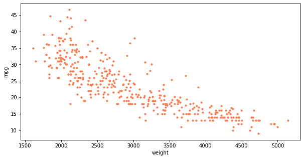
# sns 산점도 fig = plt.figure(figsize = (10,5)) ax1 = fig.add_subplot(1,2,1) ax2 = fig.add_subplot(1,2,2) sns.regplot(x='weight', y='mpg', data =ndf, ax=ax1) sns.regplot(x='weight', y='mpg', data =ndf, ax=ax2, fit_reg=False) # 회귀선 미표시 plt.show()
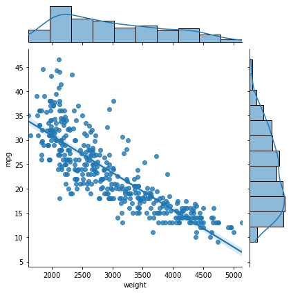
# joinplot sns.jointplot(x='weight', y='mpg', data =ndf) sns.jointplot(x='weight', y='mpg', kind = 'reg', data =ndf) plt.show()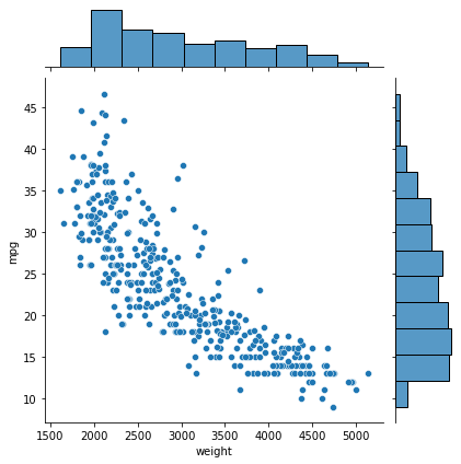
# seaborn pairplot sns.pairplot(ndf, kind = 'reg') plt.show()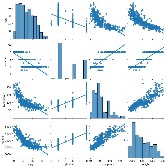
# 독립변수 여러개 x = ndf[['weight']] print(type(x)) # 종속변수 1개 y = ndf['mpg'] print(type(y)) # <class 'pandas.core.frame.DataFrame'> # <class 'pandas.core.series.Series'>
from sklearn.model_selection import train_test_split x_train, x_test, y_train, y_test = train_test_split(x, y, test_size=0.3, random_state = 10) print(len(x_train)) # 274 print(len(y_train)) # 274
from sklearn.linear_model import LinearRegression lr = LinearRegression() # 훈련 독립변수, 정답 종속변수 lr.fit(x_train, y_train) LinearRegression()
r_square = lr.score(x_test, y_test) print(r_square) # 0.6822458558299325
# 기울기 print('기울기 a', lr.coef_) print('절편 b', lr.intercept_) 기울기 a [-0.00775343] 절편 b 46.7103662572801
y_hat = lr.predict(x) plt.figure(figsize=(10,5)) ax1 = sns.kdeplot(y, label='y') ax2 = sns.kdeplot(y_hat, label='y_hat', ax=ax1) plt.legend() plt.show()
# 단순회귀분석 : 두변수간 관계를 직선으로 분석
# 다항회귀분석 : 회귀선을 곡선으로 더 높은 정확도
from sklearn.preprocessing import PolynomialFeatures poly = PolynomialFeatures(degree=2) x_train_poly = poly.fit_transform(x_train) print('원데이터 :', x_train.shape) print('2차항 변환 데이터 :', x_train_poly.shape) # 원데이터 : (274, 1) # 2차항 변환 데이터 : (274, 3)
pr = LinearRegression() pr.fit(x_train_poly, y_train) x_test_poly = poly.fit_transform(x_test) r_square = pr.score(x_test_poly, y_test) y_hat_test = pr.predict(x_test_poly) print('기울기 a', pr.coef_) print('절편 b', pr.intercept_) # 기울기 a [ 0.00000000e+00 -1.85768289e-02 1.70491223e-06] # 절편 b 62.58071221576951
# 산점도 그리기 fig = plt.figure(figsize=(10,5)) ax = fig.add_subplot(1,1,1) ax.plot(x_train, y_train, 'o', label = 'Train Data') ax.plot(x_test, y_hat_test, 'r+', label = 'Predicted Value') ax.legend(loc = 'best') plt.xlabel('weight') plt.ylabel('mpg') plt.show()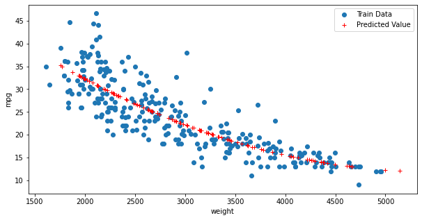
x_poly = poly.fit_transform(x) y_hat = pr.predict(x_poly) plt.figure(figsize = (10,5)) ax1 = sns.kdeplot(y, label='y') ax2 = sns.kdeplot(y_hat, label='y_hat', ax = ax1) plt.legend() plt.show()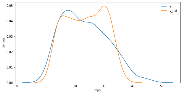
# 단순회귀분석 : 독립변수, 종속변수가 한개일때
# 다중 회귀분석 : 독립변수가 여러개일 경우
# y = b + a1*x1 + a2*x2 +...+an*xn
from sklearn.linear_model import LinearRegression lr = LinearRegression() x = ndf[['cylinders', 'horsepower', 'weight']] # 다중회귀분석 y = ndf['mpg'] x_train, x_test, y_train, y_test = train_test_split(x, y, test_size=0.3, random_state = 10)
lr.fit(x_train, y_train) r_square = lr.score(x_test, y_test) print('결정계수 :', r_square) # 결정계수 : 0.6939048496695597
print('기울기 a', lr.coef_) print('절편 b', lr.intercept_) # 기울기 a [-0.60691288 -0.03714088 -0.00522268] # 절편 b 46.41435126963407
y_hat = lr.predict(x_test)
plt.figure(figsize = (10,5)) ax1 = sns.kdeplot(y_test, label='y_test') ax2 = sns.kdeplot(y_hat, label='y_hat', ax = ax1) plt.legend() plt.show()
y_hat = lr.predict(x) plt.figure(figsize = (10,5)) ax1 = sns.kdeplot(y, label='y') ax2 = sns.kdeplot(y_hat, label='y_hat', ax = ax1) plt.legend() plt.show()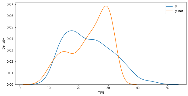
x = [[10], [5], [9], [7]] y = [100, 50, 90, 77] lr = LinearRegression() lr.fit(x,y) result =lr.predict([[7]]) plt.figure(figsize = (10,5)) ax1 = sns.kdeplot(y, label='y')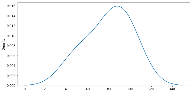
반응형
'Data_Science > Data_Analysis_Py' 카테고리의 다른 글
| 24. 위스콘신 유방안데이터 분석 || DT (0) | 2021.11.24 |
|---|---|
| 23. titanic 분류 예측 | KNN, SVM (0) | 2021.11.24 |
| 21. 서울시 범죄율 분석 || MinMaxscalimg (0) | 2021.11.24 |
| 20. 서울시 인구분석 || 다중회귀 (0) | 2021.11.23 |
| 19. 세계음주데이터2 (0) | 2021.11.23 |