import matplotlib
len(dir(matplotlib))
# 165

import matplotlib.pyplot as plt
len(dir(matplotlib))  # colab에서는 matplotlib이나 matplotlib.pyplot이나 똑같이 나오네요
# 165

!pip list # matplotlib version = 3.2.2
!python --version
Image
Image는 2차원의 함수로 정의 한다
Image는 공간에 어떤한 값을 넣었을 때 이 값에 대한 강도를 나타낸다
Color image는 3개 이상 값의 조합으로 두 좌표에 대한 강도를 나타낸다
어떻게 강도를 표현하느냐에 따라 함수가 달라질 수 있다
특히 함수가 한정적일 경우 디지털 이미지라고 부른다
직사각형 형태의 어떤 값으로 강도를 나타낸다
정의 자체는 함수이지만 그 함수를 좌표계로 구성되어 있는 array로 표현할 수 있다
Image의 두 종류
1. 벡터 이미지
- 각각 좌표에 대한 함수가 아니라 이미지 자체를 함수로 표현 한 것
- 점과 점을 연결해 수학적 원리로 그림을 그려 표현하는 방식이다
- 이미지의 크기를 늘리고 줄여도 손상되지 않는다
- 사진과 같은 복잡한 그림을 표현하려면 컴퓨터에 엄청난 부담을 주기 때문에 웹에서는 잘 사용되지 않는다
- 최근에는 컴퓨터 하드웨어의 발달로 웹사이트의 로고 및 아이콘 표시에 벡터 그래픽이 사용되고 있다
- ex) ai, eps, svg
2. 비트맵 이미지
- 서로 다른 점(픽셀)들의 조합으로 그려지는 이미지 표현 방식이다
- 비트맵 이미지는 크기를 늘리거나 줄이면 원본 이미지에 손상되어 번져 보인다
- 컴퓨터에 부담을 덜 주는 구조를 갖고 있기 때문에, 웹에서 이미지를 표시할 때는 주로 비트맵 이미지를 사용한다
- ex) jpg, jpeg, png, gif
색을 표현하는 두 가지 방식
1. HSV
- 밝기로 구분한다
- 색상(Hue), 채도(Saturation), 명도(Value)의 좌표를 써서 특정한 색을 지정한다
2. RGB
- 세가지 색이 섞여서 색을 표현한다
- 3장의 array가 합쳐진 것이다
비트맵 이미지를 표현하는 단위
1. Pixel @@@ 추가 설명
- 픽셀은 상대적 크기로 표현한다
- 픽셀은 정사각형으로 표현한다
- ppi가 클수록 1인치당 픽셀의 밀도가 더 높고 더 선명하게 보인다
2. Voxel
- 3차원 이미지에서는 voxel이라고 한다
이미지 처리를 위한 사전단계
1. Image파일을 바이너리 형태로 불러온다
2. image를 array로 바꿔준다
with open('Elon.jpg', 'rb') as f: # 기본 옵션 r은 unicode형식으로 불러온다  / rb는 바이너리로 불러온다
  print(f.read())                 # 파이썬에서는 이미지는 불러올수는 있지만 각각의 값이 어떤 색을 표현하는지 해석할 수 없다

#  b'\xff\xd8\xff\xe1\x00\x18Exif\x00\x00II*\x00\x08\x00\x00\x00\x00\x00\x00\x00\x00\x00\x00\x00\xff\xec\x00\x11Ducky\x00\x01\x00\x04...
import tensorflow as tf
im = tf.io.read_file('Elon.jpg') # vectorization으로 불러온다 / array연산을 최적화 하도록 불러온다
im
# <tf.Tensor: shape=(), dtype=string, numpy=b'\xff\xd8\xff\xe1\x00\x18Exif\x00\x00II*\x00\x08\x00\x00\x00\x00\x00\x00\x00\x00\x00\x0# .numpy() 하면 기타정보 빼고 내용만 보여줌
im.numpy()
# b'\xff\xd8\xff\xe1\x00\x18Exif\x00\x00II*\x00\x08\x00\x00\x00\x00\x00\x00\x00\x00\x00\x00\x00\xff\xec\x00\x11Ducky\x00\x01\x00\x04t = tf.image.decode_gif(im) # 바이너리 값을 해석해준다
t
# <tf.Tensor: shape=(1, 600, 960, 3), dtype=uint8, numpy=
# array([[[[ 4, 3, 9],
# [ 3, 2, 10],
# [ 4, 3, 11],
...,t = tf.image.decode_image(im)
t
# <tf.Tensor: shape=(600, 960, 3), dtype=uint8, numpy=
# array([[[ 4, 3, 9],
# [ 3, 2, 10],
# [ 4, 3, 11],import cv2
cv2.imread('Elon.jpg', ) # OpenCV는 BGR로 불러온다 / python으로 불러오는 것과 opencv로 불러오는 것은 편의성 옵션의 차이일 뿐이다
# array([[[12, 4, 5],
# [10, 2, 3],
# [11, 2, 5],s = cv2.imread('Elon.jpg', )
s.dtype # int이기 때문에 color에서 부호가 없다 / 2^8 = 256 => 0~255까지로 강도를 표현한다
# dtype('uint8')이미지를 불러올 때 tensor가 좋은 점은 gpu연산이 가능하기 때문에 대용량 이미지를 더 빠르게 불러올 수 있다
import matplotlib.pyplot as plt
plt.figure(figsize=(10,10))
plt.imshow(t) # array를 image로 해석하는 방법을 제공한다 / version 때문에 tensor를 직접 표현 못할 수 있다. 혹시 안된다면 colabd으로 사용해 보는 것을 추천한다
plt.colorbar(); # 컬러바 표시하기
plt.axis('off'); # 좌표 축 없애기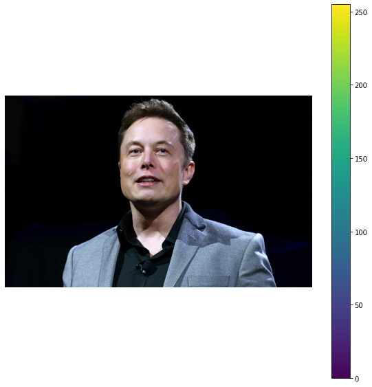
State machine
State Machine은 외부 입력에 따라 시스템의 상태가 결정되고,
이 상태와 입력에 의해서 시스템의 동작이 결정되는 시스템이다.
[특징]
1. 변수가 없다
2. figure안에 axes가 포함되어 있다. 그리고 plt.axes만 실행하면 plt.figure의 default값으로 자동실행 된다
3. 변수를 지정하지 않아도 상태를 보고 자동적으로 만들어 준다
# 같은 셀안에서 실행하면
plt.figure();
plt.axes([0.5,0.5,1,1]); # figure 안에서 좌표형태로 보여준다
plt.plot([4,5,4]);
plt.axes([0,0,0.5,0.5]);
plt.plot([4,5,4]);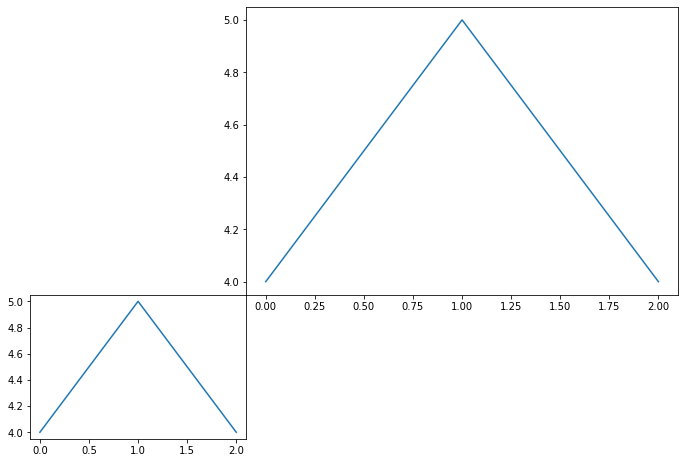
plt.axes([0,0,0.5,0.5])
# plt.figure()
# plt.axes()
plt.plot([1,2,3]) # plot만 하면 figure, axes default값으로 자동 지정된다

s = t / 255
t.dtype
# tf.uint8

s.dtype
# tf.float32

plt.imshow(s) # 이미지를 구성하는 값들은 상대적인 개념이기 때문에 특정 값을 기준으로 나누어도 사람이 볼때는 똑같은 이미지로 볼 수 있다
im = tf.io.read_file('Elon.jpg')
t = tf.image.decode_image(im)
ss = tf.cast(t, 'float32')

ss.dtype
# tf.float32

sss = (ss/127.5) -1 # -1에서 1 사이로 변환해주는 방법 / 가장 큰 값이 255이기 때문에 절반으로 나누고 1을 빼면 -1과 1 사이의 값으로 구성된다
import numpy as np
np.min(sss)
# -1.0

plt.imshow(sss) # imshow는 -1값은 표현하지 못하기 때문에 달라 보인다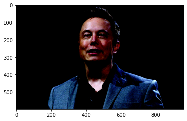
plt.imshow(sss - 1)
sss.shape
# TensorShape([600, 960, 3])

sss[...,0][..., tf.newaxis]
# <tf.Tensor: shape=(600, 960, 1), dtype=float32, numpy=
# array([[[-0.96862745],
#         [-0.9764706 ],
#         [-0.96862745],
#         ...,
t[...,2] # color 이미지에서 채널 하나 빼면 흑백이 된다 / color는 각 픽셀당 3가지 값으로 표현해야 한다
# <tf.Tensor: shape=(600, 960), dtype=uint8, numpy=
# array([[ 9, 10, 11, ..., 0, 0, 0],
# [ 8, 10, 11, ..., 0, 0, 0],
# [ 9, 10, 11, ..., 0, 0, 0],
# ...,
# [ 9, 11, 13, ..., 11, 11, 12],
# [ 9, 11, 10, ..., 12, 12, 12],
# [10, 11, 10, ..., 14, 14, 14]], dtype=uint8)>plt.imshow(t[...,1]) # (0,1), (0,255) / 흑백 이미지는 기본 colormap으로 표현 / 색깔정보가 없으면 기본 색으로 입혀준다 /imshow는 default를 color로 간주한다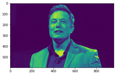
plt.imshow(t[...,1], cmap='gray') # 숫자 값이 크면 클 수록 밝게 표현한다
plt.imshow(t[...,1], cmap='gray_r') # 숫자 값이 크면 클 수록 어둡게 표현한다
plt.imshow(t[...,1], cmap=plt.cm.Reds)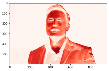
plt.imshow(t[...,1], cmap=plt.cm.Reds_r)
import matplotlib
len(dir(matplotlib))
# 165

import matplotlib.pyplot as plt
len(dir(matplotlib))  # colab에서는 matplotlib이나 matplotlib.pyplot이나 똑같이 나오네요
# 165

!pip list # matplotlib version = 3.2.2
!python --version
# Python 3.7.11
Monkey patch
한국에서는 잠수함 패치라고 부르고 영어권에서는 게릴라 패치, 고릴라 패치, 몽키 패치라고 부른다 런타임상에서 함수, 메소드, 속성을 바꾸는 패치
from PIL import Image # 파이썬 스럽게 이미지를 처리해주는 라이브러리(일반인대상으로 가장 많이 사용한다)
Image.open('Elon.jpg')
im = Image.open('Elon.jpg')
dir(im) # numpy 방식이 아닌 numpy 호환 형태로 데이터를 갖고 있다
['_Image__transformer',
 '__array_interface__',
 '__class__',
 '__copy__',
 '__delattr__',
 '__dict__',
 '__dir__',
 '__doc__',
 '__enter__',
 '__eq__',
 '__exit__',
 '__format__',
 '__ge__',
 '__getattribute__',
 '__getstate__',
 '__gt__',
 '__hash__',
 '__init__',
 '__init_subclass__',
 '__le__',
 '__lt__',
 '__module__',
 '__ne__',
 '__new__',
 '__reduce__',
 '__reduce_ex__',
 '__repr__',
 '__setattr__',
 '__setstate__',
 '__sizeof__',
 '__str__',
 '__subclasshook__',
 '__weakref__',
 '_close_exclusive_fp_after_loading',
 '_copy',
 '_crop',
 '_dump',
 '_ensure_mutable',
 '_exclusive_fp',
 '_exif',
 '_expand',
 '_get_safe_box',
 '_getexif',
 '_getmp',
 '_min_frame',
 '_new',
 '_open',
 '_repr_png_',
 '_seek_check',
 '_size',
 'alpha_composite',
 'app',
 'applist',
 'bits',
 'category',
 'close',
 'convert',
 'copy',
 'crop',
 'custom_mimetype',
 'decoderconfig',
 'decodermaxblock',
 'draft',
 'effect_spread',
 'entropy',
 'filename',
 'filter',
 'format',
 'format_description',
 'fp',
 'frombytes',
 'fromstring',
 'get_format_mimetype',
 'getbands',
 'getbbox',
 'getchannel',
 'getcolors',
 'getdata',
 'getexif',
 'getextrema',
 'getim',
 'getpalette',
 'getpixel',
 'getprojection',
 'height',
 'histogram',
 'huffman_ac',
 'huffman_dc',
 'icclist',
 'im',
 'info',
 'layer',
 'layers',
 'load',
 'load_djpeg',
 'load_end',
 'load_prepare',
 'load_read',
 'mode',
 'offset',
 'palette',
 'paste',
 'point',
 'putalpha',
 'putdata',
 'putpalette',
 'putpixel',
 'pyaccess',
 'quantization',
 'quantize',
 'readonly',
 'reduce',
 'remap_palette',
 'resize',
 'rotate',
 'save',
 'seek',
 'show',
 'size',
 'split',
 'tell',
 'thumbnail',
 'tile',
 'tobitmap',
 'tobytes',
 'toqimage',
 'toqpixmap',
 'tostring',
 'transform',
 'transpose',
 'verify',
 'width']
dir(im.getdata())
['__class__',
'__delattr__',
'__dir__',
'__doc__',
'__eq__',
'__format__',
'__ge__',
'__getattribute__',
'__getitem__',
'__gt__',
'__hash__',
'__init__',
'__init_subclass__',
'__le__',
'__len__',
'__lt__',
'__ne__',
'__new__',
'__reduce__',
'__reduce_ex__',
'__repr__',
'__setattr__',
'__sizeof__',
'__str__',
'__subclasshook__',
'bands',
'box_blur',
'chop_add',
'chop_add_modulo',
'chop_and',
'chop_darker',
'chop_difference',
'chop_hard_light',
'chop_invert',
'chop_lighter',
'chop_multiply',
'chop_or',
'chop_overlay',
'chop_screen',
'chop_soft_light',
'chop_subtract',
'chop_subtract_modulo',
'chop_xor',
'color_lut_3d',
'convert',
'convert2',
'convert_matrix',
'convert_transparent',
'copy',
'crop',
'effect_spread',
'entropy',
'expand',
'fillband',
'filter',
'gaussian_blur',
'getband',
'getbbox',
'getcolors',
'getextrema',
'getpalette',
'getpalettemode',
'getpixel',
'getprojection',
'histogram',
'id',
'isblock',
'mode',
'modefilter',
'new_block',
'offset',
'paste',
'pixel_access',
'point',
'point_transform',
'ptr',
'putband',
'putdata',
'putpalette',
'putpalettealpha',
'putpalettealphas',
'putpixel',
'quantize',
'rankfilter',
'reduce',
'resize',
'save_ppm',
'setmode',
'size',
'split',
'transform2',
'transpose',
'unsafe_ptrs',
'unsharp_mask']im_ = np.array(im)
plt.imshow(im_)
tf.keras.preprocessing.image.load_img('Elon.jpg')
i  = tf.keras.preprocessing.image.load_img('Elon.jpg') # tensorflow, pytorch는 내부적으로 PIL 사용한다
type(i)
# PIL.JpegImagePlugin.JpegImageFile
(X_train, y_train), (X_test, y_test) = tf.keras.datasets.mnist.load_data()
# Downloading data from https://storage.googleapis.com/tensorflow/tf-keras-datasets/mnist.npz
# 11493376/11490434 [==============================] - 0s 0us/step
# 11501568/11490434 [==============================] - 0s 0us/step

plt.imshow(X_train[100])
np.set_printoptions(formatter={'int': '{:>01d}'.format}, linewidth=80) # int 데이터일 경우에 한 자리로 표현해 준다
print(X_train[100])
[[0 0 0 0 0 0 0 0 0 0 0 0 0 0 0 0 0 0 0 0 0 0 0 0 0 0 0 0]
 [0 0 0 0 0 0 0 0 0 0 0 0 0 0 0 0 0 0 0 0 0 0 0 0 0 0 0 0]
 [0 0 0 0 0 0 0 0 0 0 0 0 0 0 0 0 0 0 0 0 0 0 0 0 0 0 0 0]
 [0 0 0 0 0 0 0 0 0 0 0 0 0 0 0 0 0 0 0 0 0 0 0 0 0 0 0 0]
 [0 0 0 0 0 0 0 0 0 0 0 0 0 0 0 0 0 0 0 0 0 0 0 0 0 0 0 0]
 [0 0 0 0 0 0 0 0 0 0 0 0 0 0 0 0 0 0 0 0 0 0 0 0 0 0 0 0]
 [0 0 0 0 0 0 0 0 0 0 0 0 0 2 18 46 136 136 244 255 241 103 0 0 0 0 0 0]
 [0 0 0 0 0 0 0 0 0 0 0 15 94 163 253 253 253 253 238 218 204 35 0 0 0 0 0 0]
 [0 0 0 0 0 0 0 0 0 0 0 131 253 253 253 253 237 200 57 0 0 0 0 0 0 0 0 0]
 [0 0 0 0 0 0 0 0 0 0 155 246 253 247 108 65 45 0 0 0 0 0 0 0 0 0 0 0]
 [0 0 0 0 0 0 0 0 0 0 207 253 253 230 0 0 0 0 0 0 0 0 0 0 0 0 0 0]
 [0 0 0 0 0 0 0 0 0 0 157 253 253 125 0 0 0 0 0 0 0 0 0 0 0 0 0 0]
 [0 0 0 0 0 0 0 0 0 0 89 253 250 57 0 0 0 0 0 0 0 0 0 0 0 0 0 0]
 [0 0 0 0 0 0 0 0 0 0 89 253 247 0 0 0 0 0 0 0 0 0 0 0 0 0 0 0]
 [0 0 0 0 0 0 0 0 0 0 89 253 247 0 0 0 0 0 0 0 0 0 0 0 0 0 0 0]
 [0 0 0 0 0 0 0 0 0 0 89 253 247 0 0 0 0 0 0 0 0 0 0 0 0 0 0 0]
 [0 0 0 0 0 0 0 0 0 0 21 231 249 34 0 0 0 0 0 0 0 0 0 0 0 0 0 0]
 [0 0 0 0 0 0 0 0 0 0 0 225 253 231 213 213 123 16 0 0 0 0 0 0 0 0 0 0]
 [0 0 0 0 0 0 0 0 0 0 0 172 253 253 253 253 253 190 63 0 0 0 0 0 0 0 0 0]
 [0 0 0 0 0 0 0 0 0 0 0 2 116 72 124 209 253 253 141 0 0 0 0 0 0 0 0 0]
 [0 0 0 0 0 0 0 0 0 0 0 0 0 0 0 25 219 253 206 3 0 0 0 0 0 0 0 0]
 [0 0 0 0 0 0 0 0 0 0 0 0 0 0 0 0 104 246 253 5 0 0 0 0 0 0 0 0]
 [0 0 0 0 0 0 0 0 0 0 0 0 0 0 0 0 0 213 253 5 0 0 0 0 0 0 0 0]
 [0 0 0 0 0 0 0 0 0 0 0 0 0 0 0 0 26 226 253 5 0 0 0 0 0 0 0 0]
 [0 0 0 0 0 0 0 0 0 0 0 0 0 0 0 0 132 253 209 3 0 0 0 0 0 0 0 0]
 [0 0 0 0 0 0 0 0 0 0 0 0 0 0 0 0 78 253 86 0 0 0 0 0 0 0 0 0]
 [0 0 0 0 0 0 0 0 0 0 0 0 0 0 0 0 0 0 0 0 0 0 0 0 0 0 0 0]
 [0 0 0 0 0 0 0 0 0 0 0 0 0 0 0 0 0 0 0 0 0 0 0 0 0 0 0 0]]
plt.imshow(i)
plt.annotate('0', xy=(0,0))
# Text(0, 0, '0')
def visualize_bw(img):
  w, h = img.shape
  plt.figure(figsize=(10,10))
  plt.imshow(img, cmap='binary') # binary는 작은 숫자가 밝게 / gray는 큰 숫자가 밝게
  for i in range(w):
    for j in range(h):
      x = img[j,i]
      plt.annotate(x, xy=(i,j), horizontalalignment='center', verticalalignment='center', color = 'black' if x <= 128 else 'white') # 점 하나당 대체 시킨다

visualize_bw(X_train[0])
Image processing
input image가 어떠한 함수에 의해 새로운 image가 output으로 나오는 것
array연산을 통해서 새로운 형태의 image를 만들어 내는 것
visualize_bw(X_train[5][::-1])
# 뒤집기
visualize_bw(X_train[5][4:24,4:24])
# 잘라내기
visualize_bw(np.flipud(X_train[5])) # flipud => 이미지 뒤집기
# 크기가 (20,20)인 흑백 이미지 생성
visualize_bw(np.ones((20,20)))
'Computer_Science > Visual Intelligence' 카테고리의 다른 글
| 8일차 - Image 처리 (3) (1) | 2021.09.21 |
|---|---|
| 7일차 - Image 처리 (2) (0) | 2021.09.21 |
| 5일차 - 영상 데이터 처리를 위한 Array 프로그래밍 + image 처리 (0) | 2021.09.18 |
| 4일차 - 영상 데이터 처리를 위한 객체지향 프로그래밍 (0) | 2021.09.18 |
| 3일차 - 영상 데이터 처리를 위한 객체지향 프로그래밍 (0) | 2021.09.18 |