728x90
반응형
Image 처리
import tensorflow as tf
im = tf.io.read_file('people.jpg')
im = tf.image.decode_jpeg(im)
im
# <tf.Tensor: shape=(540, 540, 3), dtype=uint8, numpy=
# array([[[200, 188, 176],
#         [202, 190, 178],
#         [204, 192, 180],
#         ...,
상황에 따라 알맞은 라이브러리를 사용하면 된다
from scipy import ndimage # 기본적인 이미지 처리 할 수 있다
from scipy import io
import imageio # image를 읽고 저장하는 기능만 제공한다
import numpy as np
import scipy # low level이기 때문에 전문가들이 주로 사용한다 / image processing에 초첨이 맞추어져 있다
# scipy-toolkit => scipy에서 파생되어 사용자 친화적인 high level인 라이브러리가 생겼다
# scipy-toolkit image => scikit-image
# scipy-toolkit machine learning => scikit-learn
# opencv => Practical
import cv2 # computer vision에 초점이 맞추어 져있다 / image array 구조가 Numpy와 다르다
import matplotlib.pyplot as plt
from PIL import Image  # pythonic한 image 처리 라이브러리
from skimage import io
import PIL

# !pip install -U opencv-python # opecnv 설치 / colab에서 하시면 설치하지 않으셔도 됩니다 / 파이썬 기반의 opencv는 한글처리 기능이 지원되지 않는다
!pip list
Package                       Version
----------------------------- --------------
absl-py                       0.12.0
alabaster                     0.7.12
albumentations                0.1.12
altair                        4.1.0
appdirs                       1.4.4
argcomplete                   1.12.3
argon2-cffi                   21.1.0
arviz                         0.11.2
astor                         0.8.1
astropy                       4.3.1
astunparse                    1.6.3
atari-py                      0.2.9
atomicwrites                  1.4.0
attrs                         21.2.0
audioread                     2.1.9
autograd                      1.3
Babel                         2.9.1
backcall                      0.2.0
beautifulsoup4                4.6.3
bleach                        4.0.0
blis                          0.4.1
bokeh                         2.3.3
Bottleneck                    1.3.2
branca                        0.4.2
bs4                           0.0.1
...
dir(ndimage)
dir(io)
dir(imageio)
['RETURN_BYTES',
'__builtins__',
'__cached__',
'__doc__',
'__file__',
'__loader__',
'__name__',
'__package__',
'__path__',
'__spec__',
'__version__',
'core',
'formats',
'get_reader',
'get_writer',
'help',
'imread',
'imsave',
'imwrite',
'mimread',
'mimsave',
'mimwrite',
'mvolread',
'mvolsave',
'mvolwrite',
'plugins',
'read',
'save',
'show_formats',
'volread',
'volsave',
'volwrite']imageio.formats # 95가지 image format을 지원한다
# <imageio.FormatManager with 96 registered formats>imageio.imread('people.jpg')
# Array([[[201, 189, 177],
# [203, 191, 179],
# [204, 192, 180],
# ...,type(imageio.imread('people.jpg'))
# imageio.core.util.Array
issubclass(type(imageio.imread('people.jpg')), np.ndarray)
# True
imageio.core.util.Array.__base__ # 부모 클래스
# numpy.ndarray
imageio.core.util.Array.mro()
# [imageio.core.util.Array, numpy.ndarray, object]OpenCV
opencv c버전은 c/c++ 관례를 따른다
dir(cv2)
['',
 'ACCESS_FAST',
 'ACCESS_MASK',
 'ACCESS_READ',
 'ACCESS_RW',
 'ACCESS_WRITE',
 'ADAPTIVE_THRESH_GAUSSIAN_C',
 'ADAPTIVE_THRESH_MEAN_C',
im2 = cv2.imread('people.jpg')
plt.imshow(im2)
RGB로 처리하는 것이 선명하게 잘 보여주지만 비용이 많이 들기 때문에
저가 모니터는 BGR 처리를 한다
opencv는 BGR 배열로 표현해준다
plt.imshow(im2[...,::-1])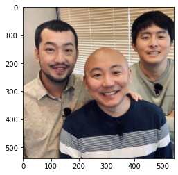
im3 = cv2.imread('people.jgp') # 확장자를 잘 못 적어도 에러가 나지 않는다
plt.imshow(im)
im1 = cv2.imread('people.jpg')    # 3차원으로 불러온다 / 컬러 이미지

im2 = cv2.imread('people.jpg', 0) # 2차원으로 불러온다 / 흑백 이미지

im1.shape, im2.shape
# ((540, 540, 3), (540, 540))

im3 = cv2.imread('people.jpg', 100)
im3.shape
# (135, 135, 3)
dir(cv2) # 대문자는 옵션이다
for i in dir(cv2):
if 'imread' in i:
print(i)
# imread
# imreadmultifor i in dir(cv2):
if 'IMREAD' in i:
print(i, getattr(cv2, i)) # 옵션
IMREAD_ANYCOLOR 4
IMREAD_ANYDEPTH 2
IMREAD_COLOR 1
IMREAD_GRAYSCALE 0
IMREAD_IGNORE_ORIENTATION 128
IMREAD_LOAD_GDAL 8
IMREAD_REDUCED_COLOR_2 17
IMREAD_REDUCED_COLOR_4 33
IMREAD_REDUCED_COLOR_8 65
IMREAD_REDUCED_GRAYSCALE_2 16
IMREAD_REDUCED_GRAYSCALE_4 32
IMREAD_REDUCED_GRAYSCALE_8 64
IMREAD_UNCHANGED -1Saturated / Modular 연산
im = cv2.imread('people.jpg')
im
# array([[[177, 189, 201],
#         [179, 191, 203],
#         [180, 192, 204],
#         ...,
cv2.add(im, im) # 가장 큰 값이 255이기 때문에 합이 255를 넘어가면 saturated 연산이 적용된다
array([[[255, 255, 255],
[255, 255, 255],
[255, 255, 255],
...,
[252, 255, 255],
[254, 255, 255],
[255, 255, 255]],(177+177) - 256 # im의 첫번쨰 값: 177 / 177 + 177이 255을 초과 했기 때문에 modular연산에서는 256(dtype이 8이었기 때문에 2^8)을 빼는 연산을 한다
# 98im.dtype
# dtype('uint8')
np.add(im, im) # modular 연산
# array([[[ 98, 122, 146],
# [102, 126, 150],
# [104, 128, 152],
# ...,Basic Operation
im[100,40]
# array([183, 198, 207], dtype=uint8)

im[100,40,2]
# 207

im.item(100,40,2)
# 207

im[100,40,2] = 100

im.item(100,40,2)
# 100

im.itemset((100,40,2), 207) # 값 조정
im.item(100,40,2)
# 207

im[200:30,330:2]

array([], shape=(0, 0, 3), dtype=uint8)
plt.imshow(im[...,::-1])
Channel
im_cv = cv2.imread('people.jpg')
im[...,2]
array([[201, 203, 204, ..., 193, 194, 196],
       [200, 202, 203, ..., 201, 203, 204],
       [199, 201, 202, ..., 209, 210, 211],
       ...,
       [114, 112, 120, ...,  98, 109, 114],
       [116, 112, 120, ...,  96, 103, 106],
       [111, 107, 115, ..., 102, 103, 103]], dtype=uint8)
len(cv2.split(im))
# 3
plt.imshow(im_cv)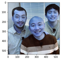
B, G, R = cv2.split(im_cv) # function 방식
im_cv = cv2.merge((R,G,B))
plt.imshow(im_cv)
for i in dir(cv2):
  if 'COLOR_BGR2' in i:
    print(i, getattr(cv2, i))

COLOR_BGR2BGR555 22
COLOR_BGR2BGR565 12
COLOR_BGR2BGRA 0
COLOR_BGR2GRAY 6
COLOR_BGR2HLS 52
COLOR_BGR2HLS_FULL 68
COLOR_BGR2HSV 40
COLOR_BGR2HSV_FULL 66
COLOR_BGR2LAB 44
COLOR_BGR2LUV 50
COLOR_BGR2Lab 44
COLOR_BGR2Luv 50
COLOR_BGR2RGB 4
COLOR_BGR2RGBA 2
COLOR_BGR2XYZ 32
COLOR_BGR2YCR_CB 36
COLOR_BGR2YCrCb 36
COLOR_BGR2YUV 82
COLOR_BGR2YUV_I420 128
COLOR_BGR2YUV_IYUV 128
COLOR_BGR2YUV_YV12 132
cv2.cvtColor(im_cv, cv2.COLOR_BGR2GRAY) # 색공간 바꾸기
array([[187, 189, 190, ..., 152, 153, 155],
[186, 188, 189, ..., 160, 162, 163],
[185, 187, 188, ..., 170, 171, 172],
...,
[100, 96, 103, ..., 119, 130, 135],
[100, 96, 103, ..., 119, 126, 129],
[ 95, 91, 98, ..., 125, 126, 126]], dtype=uint8)cv2.cvtColor(im_cv, cv2.COLOR_BGR2RGB)
array([[[177, 189, 201],
[179, 191, 203],
[180, 192, 204],
...,for i in dir(cv2):
if 'BORDER_' in i :
print(i, getattr(cv2, i))
BORDER_CONSTANT 0
BORDER_DEFAULT 4
BORDER_ISOLATED 16
BORDER_REFLECT 2
BORDER_REFLECT101 4
BORDER_REFLECT_101 4
BORDER_REPLICATE 1
BORDER_TRANSPARENT 5
BORDER_WRAP 3plt.imshow(cv2.copyMakeBorder(im_cv, 10,10,10,10,0))
plt.imshow(np.pad(im_cv,[(10,10),(10,10),(0,0)], mode='constant'))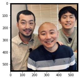
PIL
PIL은 이미지 파일 자체에 대한 내용도 알 수 있다
meta data에 대한 정보가 필요할떄 유용하다
im4 = Image.open('people.jpg') # mutable 방식 지원
plt.imshow(im4)
b = np.array(im4)
Image.fromarray(b)
type(b)
# numpy.ndarray

type(im4) # 데이터 구조 자체가 numpy와 다르다 하지만 Numpy와 호환이 된다
# PIL.JpegImagePlugin.JpegImageFile

im4.format_description
# 'JPEG (ISO 10918)'

im4.getexif().keys()
# KeysView(<PIL.Image.Exif object at 0x7f424eb895d0>)
im_pil = Image.open('people.jpg')
R, G, B = im_pil.split() # method 방식
Image.merge('RGB', (R,G,B))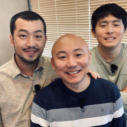
Image.merge('RGB', (B,G,R))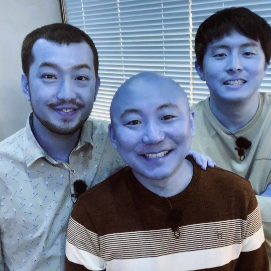
'ImageMode' in dir(PIL) # composition 방식으로 만들어짐
# True
from PIL import ImageMode
ImageMode._modes # Image.merge(mode, bands) 모드 자리에 들어 갈 수 있는 키값들
{'1': <PIL.ImageMode.ModeDescriptor at 0x7f4249d1b350>,
'CMYK': <PIL.ImageMode.ModeDescriptor at 0x7f4249d45bd0>,
'F': <PIL.ImageMode.ModeDescriptor at 0x7f4249d45d50>,
'HSV': <PIL.ImageMode.ModeDescriptor at 0x7f4249d45590>,
'I': <PIL.ImageMode.ModeDescriptor at 0x7f4249d45d90>,
'I;16': <PIL.ImageMode.ModeDescriptor at 0x7f4249d45a50>,
'I;16B': <PIL.ImageMode.ModeDescriptor at 0x7f4249d45f50>,
'I;16BS': <PIL.ImageMode.ModeDescriptor at 0x7f4249d45e90>,
'I;16L': <PIL.ImageMode.ModeDescriptor at 0x7f4249d45410>,
'I;16LS': <PIL.ImageMode.ModeDescriptor at 0x7f4249d450d0>,
'I;16N': <PIL.ImageMode.ModeDescriptor at 0x7f4249d45390>,
'I;16NS': <PIL.ImageMode.ModeDescriptor at 0x7f4249d31610>,
'I;16S': <PIL.ImageMode.ModeDescriptor at 0x7f4249d45ad0>,
'L': <PIL.ImageMode.ModeDescriptor at 0x7f4249d1bd10>,
'LA': <PIL.ImageMode.ModeDescriptor at 0x7f4249d45190>,
'LAB': <PIL.ImageMode.ModeDescriptor at 0x7f4249d45110>,
'La': <PIL.ImageMode.ModeDescriptor at 0x7f4249d457d0>,
'P': <PIL.ImageMode.ModeDescriptor at 0x7f4249d45e50>,
'PA': <PIL.ImageMode.ModeDescriptor at 0x7f4249d452d0>,
'RGB': <PIL.ImageMode.ModeDescriptor at 0x7f4249d45850>,
'RGBA': <PIL.ImageMode.ModeDescriptor at 0x7f4249d45210>,
'RGBX': <PIL.ImageMode.ModeDescriptor at 0x7f4249d45e10>,
'RGBa': <PIL.ImageMode.ModeDescriptor at 0x7f4249d45510>,
'YCbCr': <PIL.ImageMode.ModeDescriptor at 0x7f4249d45a90>}
im_pil.convert('L')
PIL은 pad를 지원하지 않는다
im_pil.width
# 540

im_pil.height
# 540

im_pil.info # meat data
# {'jfif': 257, 'jfif_density': (1, 1), 'jfif_unit': 0, 'jfif_version': (1, 1)}

im_new = Image.new('RGB',(im_pil.width + 20, im_pil.height + 20))
im_new.paste(im_pil, (20,20)) # output이 없다 / mutable 방식
im_new
from PIL import ImageOps
ImageOps.expand(im_pil, 10) # composition 방법
PIL을 사용하는 이유
tensorflow와 pytorch에서 이미지를 불러올 때 내부적으로 처리하기 때문에 알고 있어야 한다
tf.keras.preprocessing.image.load_img('people.jpg')
Scikit image
from skimage.color import rgb2gray # skimage는 BGR를 지원하지 안는다
plt.imshow(rgb2gray(im[...,::-1]))
plt.imshow(rgb2gray(im[...,::-1]), cmap='gray')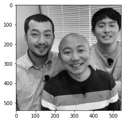
plt.imshow(np.mean(im,2))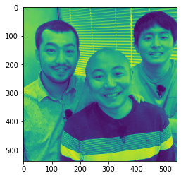
R,G,B = im[...,0], im[...,1], im[...,2]
gray = R*0.13 + G*0.15 + B*0.14
np.mean(im,2) # (im[...,0]) + im[...,1] + im[...,2]) / 3
plt.imshow(np.mean(im,2), cmap='gray')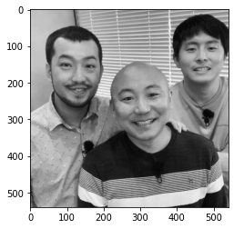
각각 이미지 처리 라이브러리에 대한 장점들
속도 차이 : opencv > numpy > PIL
im = tf.io.read_file('people.jpg')
im = tf.image.decode_jpeg(im)

im = imageio.imread('people.jpg') # Array (array 상속) / 다양한 포맷 지원 / 여러 이미지 불러올 수 있다

im = cv2.imread('people.jpg') # c/c++ style / array가 BGR로 구성되어 있다 / opencv는 gpu도 지원하기 때문에 속도가 가장 빠르다

im = Image.open('people.jpg') # numpy와 호환이 되지만 numpy format은 아니다 / PIL이 가장 느리다

plt.imread('people.jpg') # png파일 불러오지 못함
array([[[201, 189, 177],
        [203, 191, 179],
        [204, 192, 180],
        ...,
        [194, 158, 126],
from skimage import io
im = io.imread('people.jpg')
plt.imshow(im)
im = Image.open('people.jpg')
im2 = im.getdata()

type(im2)
# ImagingCore

list(im2)
'__iter__' in dir(im2)
# False

im2.__class__.mro() # ImagingCore에 __iter__가 있기때문에 반복, 순회 가능
# [ImagingCore, object]

im = Image.open('people.jpg').convert('1') # meta data를 갖고 있기때문에 가능한 방법
im.getcolors()
# [(142786, 0), (148814, 255)]
복습
Stride
a = np.arange(24).reshape(6,4) # 내부적으로는 일렬로 저장된다
a.flags # Information about the memory layout of the array.
#  C_CONTIGUOUS : True
#  F_CONTIGUOUS : False
#  OWNDATA : False
#  WRITEABLE : True
#  ALIGNED : True
#  WRITEBACKIFCOPY : False
#  UPDATEIFCOPY : False

a.dtype
# dtype('int64')

a.strides # 1차원의 array를 조립하는 가이드 라인
# (32, 8)

a.itemsize # memory 크기가 8인 정육각형
# 8

a
array([[ 0,  1,  2,  3],
       [ 4,  5,  6,  7],
       [ 8,  9, 10, 11],
       [12, 13, 14, 15],
       [16, 17, 18, 19],
       [20, 21, 22, 23]])

a.shape
# (6, 4)

a.sum(0) # axis = 0 기준으로 더한다
# array([60, 66, 72, 78])

a.sum(1) # axis = 1 기준으로 더한다
# array([ 6, 22, 38, 54, 70, 86])

b = np.arange(24).reshape(2,3,4)
b.shape
# (2, 3, 4)

b.sum(axis=1) # shape에서 index 1을 지우면 결과는 (2,4)
array([[12, 15, 18, 21],
       [48, 51, 54, 57]])

b.sum(axis=2) # shape에서 index 2를 지우면 결과는 (2,3)
array([[ 6, 22, 38],
       [54, 70, 86]])
반응형
'Computer_Science > Visual Intelligence' 카테고리의 다른 글
| 9일차 image 처리 (4) (0) | 2021.09.21 |
|---|---|
| 8일차 - Image 처리 (3) (1) | 2021.09.21 |
| 6일차 - Image 처리 (1) (0) | 2021.09.21 |
| 5일차 - 영상 데이터 처리를 위한 Array 프로그래밍 + image 처리 (0) | 2021.09.18 |
| 4일차 - 영상 데이터 처리를 위한 객체지향 프로그래밍 (0) | 2021.09.18 |