im[a,b,0] = 255 # R
im[a,b,1] = 0   # G
im[a,b,2] = 0   # B

plt.figure(figsize=(6,6))
plt.imshow(im)
Image Processing
이미지 처리란 넓은 의미에서 광학, 아날로그, 디지털 사진 혹은 영상 처리를 의미하지만,
computer vision에서는 디지털 이미지 데이터를 조작하여 원하는 데이터 형태로 변환하는 것을 의미한다.
이미지 처리 기법
1. 이미지 자르기(crop), 색상 공간(color space)변경, 이미지 깊이(image depth)변경, 확대·축소·회전·뒤집기와 같은 기하학적 변환
2. 이미지 대비·밝기·색상 밸런스 조정·선명도 변경과 같은 색 변환
3. 이미지 합성, 필터(filter, kernel, mask)를 사용한 블러링(Blurring)
4. 팽창과 침식 연산을 사용한 모폴로지(Morphology) 연산
5. 이미지 분할(Segmentation)
6. 이미지 검출(Detection)
7. 자세 추정(Pose Estimation)
8. 이미지 증강(Augmentation) 등 다양한 기법들이 있다
PIL, opencv, scikit-image등으로 이미지 처리 기법을 구현하여 원하는 이미지 형태로 변형 할 수 있다.
단순히 python 라이브러리로 이미지 검출이나, 자세 추정, 이미지 분할등 원하는 형태로 이미지를 가공 할 수 있지만
머신러닝, 딥러닝을 활용하면 조금 더 정교하고 대량의 이미지를 짧은 시간에 처리하는 것이 가능해진다.
이미지 처리를 하는 이유
이미지 데이터를 활용하여 어떠한 목적을 달성해야 할때 (머신러닝, 딥러닝을 활용하여 문제 해결을 해야 할때)
충분하지 못한 이미지 데이터를 갖고 있거나, 데이터 품질이 좋지 못할때, 데이터에 표시를 해야 할때등
여러가지 이유에서 목적을 수월하게 달성할 수 있다.
이미지 처리를 위한 python library
1. Scikit-image => Numpy style
2. OpenCV => C style
3. PIL => Python style
Scikit-Image
scikit-learn과 비슷한 명명 규칙을 따른다
skimage의 중분류
1. color # 색 변환
2. draw # 이미지내 그림 표시, 문자 표시, 좌표 그리기
from skimage.draw import line, rectangle, circle
from skimage.io import imread
import matplotlib.pyplot as plt
import numpy as np

len(line(0,0,100,100))
# 2
a, b = line(0,0,100,200) # 좌표평면에서 y축 방향은 앞 두 자리(0,0), x축은 뒤 두 자리(100,200) / 왼쪽 위(0,0)좌표에서 오른쪽 아래(100,200)좌표를 향하는 직선
a
array([ 0, 1, 1, 2, 2, 3, 3, 4, 4, 5, 5, 6, 6,
7, 7, 8, 8, 9, 9, 10, 10, 11, 11, 12, 12, 13,
13, 14, 14, 15, 15, 16, 16, 17, 17, 18, 18, 19, 19,
20, 20, 21, 21, 22, 22, 23, 23, 24, 24, 25, 25, 26,
26, 27, 27, 28, 28, 29, 29, 30, 30, 31, 31, 32, 32,
33, 33, 34, 34, 35, 35, 36, 36, 37, 37, 38, 38, 39,
39, 40, 40, 41, 41, 42, 42, 43, 43, 44, 44, 45, 45,
46, 46, 47, 47, 48, 48, 49, 49, 50, 50, 51, 51, 52,
52, 53, 53, 54, 54, 55, 55, 56, 56, 57, 57, 58, 58,
59, 59, 60, 60, 61, 61, 62, 62, 63, 63, 64, 64, 65,
65, 66, 66, 67, 67, 68, 68, 69, 69, 70, 70, 71, 71,
72, 72, 73, 73, 74, 74, 75, 75, 76, 76, 77, 77, 78,
78, 79, 79, 80, 80, 81, 81, 82, 82, 83, 83, 84, 84,
85, 85, 86, 86, 87, 87, 88, 88, 89, 89, 90, 90, 91,
91, 92, 92, 93, 93, 94, 94, 95, 95, 96, 96, 97, 97,
98, 98, 99, 99, 100, 100])
b
array([ 0, 1, 2, 3, 4, 5, 6, 7, 8, 9, 10, 11, 12,
13, 14, 15, 16, 17, 18, 19, 20, 21, 22, 23, 24, 25,
26, 27, 28, 29, 30, 31, 32, 33, 34, 35, 36, 37, 38,
39, 40, 41, 42, 43, 44, 45, 46, 47, 48, 49, 50, 51,
52, 53, 54, 55, 56, 57, 58, 59, 60, 61, 62, 63, 64,
65, 66, 67, 68, 69, 70, 71, 72, 73, 74, 75, 76, 77,
78, 79, 80, 81, 82, 83, 84, 85, 86, 87, 88, 89, 90,
91, 92, 93, 94, 95, 96, 97, 98, 99, 100, 101, 102, 103,
104, 105, 106, 107, 108, 109, 110, 111, 112, 113, 114, 115, 116,
117, 118, 119, 120, 121, 122, 123, 124, 125, 126, 127, 128, 129,
130, 131, 132, 133, 134, 135, 136, 137, 138, 139, 140, 141, 142,
143, 144, 145, 146, 147, 148, 149, 150, 151, 152, 153, 154, 155,
156, 157, 158, 159, 160, 161, 162, 163, 164, 165, 166, 167, 168,
169, 170, 171, 172, 173, 174, 175, 176, 177, 178, 179, 180, 181,
182, 183, 184, 185, 186, 187, 188, 189, 190, 191, 192, 193, 194,
195, 196, 197, 198, 199, 200])im = imread('people.jpg')
type(im) # ndarray => mutable
# numpy.ndarray
im[a,b] = 0
plt.figure(figsize=(6,6))
plt.imshow(im)
im = imread('people.jpg')
type(im) # ndarray => mutable
# numpy.ndarray

im[a,b] = 0
plt.figure(figsize=(6,6))
plt.imshow(im)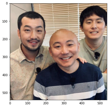
x = np.arange(24).reshape(4,6)
x[[0,1,2],[1,2,3]] # 1, 8, 15 방향의 직선 => a, b = line(0,0,100,200) 와 유사한 인덱싱
# array([ 1,  8, 15])

x
array([[ 0,  1,  2,  3,  4,  5],
       [ 6,  7,  8,  9, 10, 11],
       [12, 13, 14, 15, 16, 17],
       [18, 19, 20, 21, 22, 23]])
h, w = rectangle((20,20),(100,100))
im[h,w] = 0
# 직선과 직사각형이 이미지에 같이 표시되는 이유는 im 객체가 mutable이기 때문에 line함수와 rectangle함수가 적용된 결과가 누적된다
plt.figure(figsize=(6,6))
plt.imshow(im)
h, w = rectangle((300,300),(100,100))
im[h,w] = 0
plt.figure(figsize=(6,6))
plt.imshow(im)
im.shape
#(540, 540, 3)
im[h,w,...]
im[h,w,:] == im[h,w]
im[h,w][:]
im[h,w]
im[h,w,0] = 0
im[h,w,1] = 0 == im[h,w] = 0
im[h,w,2] = 0
좌표축 그리는 3총사
1. np.meshgrid
2. np.ogrid
3. np.mgrid
meshgrid
a = np.arange(100)
b = np.arange(100)
h,w = np.meshgrid(a,b)

grid = h + w

h.shape
# (50, 100)

w.shape
# (50, 100)

grid
array([[  0,   1,   2, ...,  97,  98,  99],
       [  1,   2,   3, ...,  98,  99, 100],
       [  2,   3,   4, ...,  99, 100, 101],
       ...,
       [ 47,  48,  49, ..., 144, 145, 146],
       [ 48,  49,  50, ..., 145, 146, 147],
       [ 49,  50,  51, ..., 146, 147, 148]])
grid.shape
# (50, 100)
plt.figure(figsize=(6,6))
plt.imshow(grid)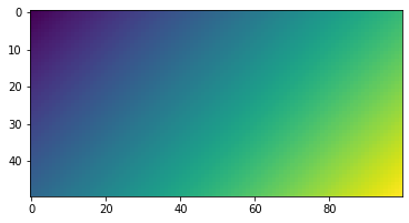
a = np.arange(100)
b = np.arange(50)
h,w = np.meshgrid(a,b)
grid = h + w

plt.figure(figsize=(6,6))
plt.scatter(w,h) # x축, y축
plt.grid()
ogrid
'__getitem__' in dir(np.ogrid) # getitem이 있으면 대괄호([])를 사용할 수 있다
# True

len(np.ogrid[0:100,0:100])
# 2


x, y = np.ogrid[0:100,0:100]
x

y
array([[ 0,  1,  2,  3,  4,  5,  6,  7,  8,  9, 10, 11, 12, 13, 14, 15,
        16, 17, 18, 19, 20, 21, 22, 23, 24, 25, 26, 27, 28, 29, 30, 31,
        32, 33, 34, 35, 36, 37, 38, 39, 40, 41, 42, 43, 44, 45, 46, 47,
        48, 49, 50, 51, 52, 53, 54, 55, 56, 57, 58, 59, 60, 61, 62, 63,
        64, 65, 66, 67, 68, 69, 70, 71, 72, 73, 74, 75, 76, 77, 78, 79,
        80, 81, 82, 83, 84, 85, 86, 87, 88, 89, 90, 91, 92, 93, 94, 95,
        96, 97, 98, 99]])

x + y
array([[  0,   1,   2, ...,  97,  98,  99],
       [  1,   2,   3, ...,  98,  99, 100],
       [  2,   3,   4, ...,  99, 100, 101],
       ...,
       [ 97,  98,  99, ..., 194, 195, 196],
       [ 98,  99, 100, ..., 195, 196, 197],
       [ 99, 100, 101, ..., 196, 197, 198]])

x.shape
(100, 1)

y.shape
(1, 100)

grid = x + y

plt.figure(figsize=(6,6))
plt.imshow(grid)
x, y = np.ogrid[0:50,0:100]
grid = x + y

plt.figure(figsize=(6,6))
plt.imshow(grid)
h,w = circle(10,10,10) # 원점 (10,10)을 중심으로 반지름이 10인 원 그리기
grid = x + y
grid[h,w] = 255

grid.shape
# (100, 100)

plt.figure(figsize=(6,6))
plt.imshow(grid) # ogrid로 만든 좌표축에 circle을 포함시켰다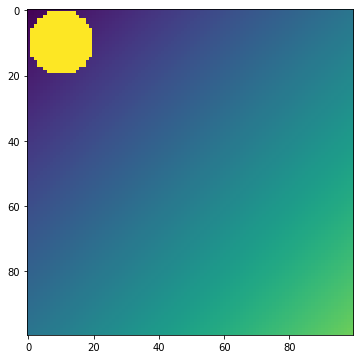
xx, yy = np.ogrid[0:10:3j,0:10:3j] # 0부터 10까지 숫자를 3등분 해서 좌표축을 만든다
grid = xx + yy
h,w = circle(1,1,1)
grid[h,w] = 10

xx
# array([[ 0.],
       [ 5.],
       [10.]])

yy
# array([[ 0.,  5., 10.]])

grid.shape
# (3, 3)

plt.figure(figsize=(6,6))
plt.imshow(grid)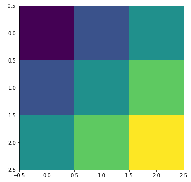
grid[...] = 0

plt.imshow(grid)
x, y = np.ogrid[0:10, 0:10]

grid = x + y

grid[2*x-y==0]
# array([ 0,  3,  6,  9, 12])

grid # y = 2x
array([[ 0,  1,  2,  3,  4,  5,  6,  7,  8,  9],
       [ 1,  2,  3,  4,  5,  6,  7,  8,  9, 10],
       [ 2,  3,  4,  5,  6,  7,  8,  9, 10, 11],
       [ 3,  4,  5,  6,  7,  8,  9, 10, 11, 12],
       [ 4,  5,  6,  7,  8,  9, 10, 11, 12, 13],
       [ 5,  6,  7,  8,  9, 10, 11, 12, 13, 14],
       [ 6,  7,  8,  9, 10, 11, 12, 13, 14, 15],
       [ 7,  8,  9, 10, 11, 12, 13, 14, 15, 16],
       [ 8,  9, 10, 11, 12, 13, 14, 15, 16, 17],
       [ 9, 10, 11, 12, 13, 14, 15, 16, 17, 18]])
x, y = np.ogrid[-10:10, -10:10]
grid = x + y
grid[...] = 0
grid[x+2*y-3 == 0] # x + 2y -3 = 0 값을 0으로 잡아 놨기 때문에 그래프를 그릴 수 없다
# array([0, 0, 0, 0, 0, 0, 0, 0, 0, 0])
# 값을 0으로 잡지 않고 했을 때는 그래프를 그릴 수 있다
grid = x + y
grid[x+2*y-3 == 0]
# array([-3, -2, -1, 0, 1, 2, 3, 4, 5, 6])
x, y = np.ogrid[-5:5, -5:5]
grid = x + y
grid
array([[-10, -9, -8, -7, -6, -5, -4, -3, -2, -1],
[ -9, -8, -7, -6, -5, -4, -3, -2, -1, 0],
[ -8, -7, -6, -5, -4, -3, -2, -1, 0, 1],
[ -7, -6, -5, -4, -3, -2, -1, 0, 1, 2],
[ -6, -5, -4, -3, -2, -1, 0, 1, 2, 3],
[ -5, -4, -3, -2, -1, 0, 1, 2, 3, 4],
[ -4, -3, -2, -1, 0, 1, 2, 3, 4, 5],
[ -3, -2, -1, 0, 1, 2, 3, 4, 5, 6],
[ -2, -1, 0, 1, 2, 3, 4, 5, 6, 7],
[ -1, 0, 1, 2, 3, 4, 5, 6, 7, 8]])
grid[x==y] # 조건식을 둘수 있다
# array([-10, -8, -6, -4, -2, 0, 2, 4, 6, 8])
x == y
# array([[ True, False, False, False, False, False, False, False, False, False],
[False, True, False, False, False, False, False, False, False, False],
[False, False, True, False, False, False, False, False, False, False],
[False, False, False, True, False, False, False, False, False, False],
[False, False, False, False, True, False, False, False, False, False],
[False, False, False, False, False, True, False, False, False, False],
[False, False, False, False, False, False, True, False, False, False],
[False, False, False, False, False, False, False, True, False, False],
[False, False, False, False, False, False, False, False, True, False],
[False, False, False, False, False, False, False, False, False, True]])
grid[x==y] = 0
grid
array([[ 0, -9, -8, -7, -6, -5, -4, -3, -2, -1],
[-9, 0, -7, -6, -5, -4, -3, -2, -1, 0],
[-8, -7, 0, -5, -4, -3, -2, -1, 0, 1],
[-7, -6, -5, 0, -3, -2, -1, 0, 1, 2],
[-6, -5, -4, -3, 0, -1, 0, 1, 2, 3],
[-5, -4, -3, -2, -1, 0, 1, 2, 3, 4],
[-4, -3, -2, -1, 0, 1, 0, 3, 4, 5],
[-3, -2, -1, 0, 1, 2, 3, 0, 5, 6],
[-2, -1, 0, 1, 2, 3, 4, 5, 0, 7],
[-1, 0, 1, 2, 3, 4, 5, 6, 7, 0]])
grid[x==y] = 255
grid # y = x / 통념상 y = x일 때 왼쪽 아래에서 오른쪽 위로 뻗는 직선이 맞지만 grid함수로 만들어진 좌표축은 y축 방향이 ↓(아래쪽 화살표) 아래로 향하기 때문에 왼쪽 위에서 오른쪽 아래로 뻗는 직선이 나온다
array([[255, -9, -8, -7, -6, -5, -4, -3, -2, -1],
[ -9, 255, -7, -6, -5, -4, -3, -2, -1, 0],
[ -8, -7, 255, -5, -4, -3, -2, -1, 0, 1],
[ -7, -6, -5, 255, -3, -2, -1, 0, 1, 2],
[ -6, -5, -4, -3, 255, -1, 0, 1, 2, 3],
[ -5, -4, -3, -2, -1, 255, 1, 2, 3, 4],
[ -4, -3, -2, -1, 0, 1, 255, 3, 4, 5],
[ -3, -2, -1, 0, 1, 2, 3, 255, 5, 6],
[ -2, -1, 0, 1, 2, 3, 4, 5, 255, 7],
[ -1, 0, 1, 2, 3, 4, 5, 6, 7, 255]])mgrid
len(np.mgrid[0:100,0:100])
# 2

a, b = np.mgrid[0:100,0:100]
aa, bb = np.mgrid[0:10:5j,0:10:5j] # 0부터 10까지 숫자를 5등분 해서 좌표축을 만든다
a
array([ 0,  1,  2,  3,  4,  5,  6,  7,  8,  9, 10, 11, 12, 13, 14, 15, 16,
       17, 18, 19, 20, 21, 22, 23, 24, 25, 26, 27, 28, 29, 30, 31, 32, 33,
       34, 35, 36, 37, 38, 39, 40, 41, 42, 43, 44, 45, 46, 47, 48, 49, 50,
       51, 52, 53, 54, 55, 56, 57, 58, 59, 60, 61, 62, 63, 64, 65, 66, 67,
       68, 69, 70, 71, 72, 73, 74, 75, 76, 77, 78, 79, 80, 81, 82, 83, 84,
       85, 86, 87, 88, 89, 90, 91, 92, 93, 94, 95, 96, 97, 98, 99])


aa
array([[ 0. ,  0. ,  0. ,  0. ,  0. ],
       [ 2.5,  2.5,  2.5,  2.5,  2.5],
       [ 5. ,  5. ,  5. ,  5. ,  5. ],
       [ 7.5,  7.5,  7.5,  7.5,  7.5],
       [10. , 10. , 10. , 10. , 10. ]])

b
array([[ 0,  1,  2, ..., 97, 98, 99],
       [ 0,  1,  2, ..., 97, 98, 99],
       [ 0,  1,  2, ..., 97, 98, 99],
       ...,
       [ 0,  1,  2, ..., 97, 98, 99],
       [ 0,  1,  2, ..., 97, 98, 99],
       [ 0,  1,  2, ..., 97, 98, 99]])

a.shape
(100, 100)

b.shape
(100, 100)

grid = a + b

plt.figure(figsize=(6,6))
plt.imshow(grid)
c, d = np.mgrid[0:10,0:10]
c + d # 안에 있는 값은 의미 없다 / 좌표축을 만들어 준다는 것이 중요하다
array([[ 0,  1,  2,  3,  4,  5,  6,  7,  8,  9],
       [ 1,  2,  3,  4,  5,  6,  7,  8,  9, 10],
       [ 2,  3,  4,  5,  6,  7,  8,  9, 10, 11],
       [ 3,  4,  5,  6,  7,  8,  9, 10, 11, 12],
       [ 4,  5,  6,  7,  8,  9, 10, 11, 12, 13],
       [ 5,  6,  7,  8,  9, 10, 11, 12, 13, 14],
       [ 6,  7,  8,  9, 10, 11, 12, 13, 14, 15],
       [ 7,  8,  9, 10, 11, 12, 13, 14, 15, 16],
       [ 8,  9, 10, 11, 12, 13, 14, 15, 16, 17],
       [ 9, 10, 11, 12, 13, 14, 15, 16, 17, 18]])


(c + d)[(0,1),(0,1)] = 0 # 흑백 이미지 / 2차원 좌표축 만드는 것
meshgrid vs ogrid vs mgrid
| mesgrid | ogrid | mgrid |
| indexer 표현 X | indexer 표현 O | indexer 표현 O |
| 행과 열이 바뀌어 표현한다 | 중복된것 줄여서작게 표현한다 | 다 표현해 준다 |
| j(n등분)를 사용 X | j(n등분)를 사용 O | j(n등분)를 사용 O |
| 비어 있는 2차원 좌표축을 그릴때 사용한다 | ||
me1, me2 = np.meshgrid(np.arange(100),np.arange(100))
og1, og2 = np.ogrid[0:100,0:100]
mg1, mg2 = np.mgrid[0:100,0:100]

np.array_equal(mg1+mg2, og1+og2) # mg1+mg2(mgrid)는 모든 수 다 표현해 준다 / or1+or2(ogrid)는 broadcasting 연산을 하도록 표현한다
# True

mg1+mg2
array([[  0,   1,   2, ...,  97,  98,  99],
       [  1,   2,   3, ...,  98,  99, 100],
       [  2,   3,   4, ...,  99, 100, 101],
       ...,
       [ 97,  98,  99, ..., 194, 195, 196],
       [ 98,  99, 100, ..., 195, 196, 197],
       [ 99, 100, 101, ..., 196, 197, 198]])

og1+og2
array([[  0,   1,   2, ...,  97,  98,  99],
       [  1,   2,   3, ...,  98,  99, 100],
       [  2,   3,   4, ...,  99, 100, 101],
       ...,
       [ 97,  98,  99, ..., 194, 195, 196],
       [ 98,  99, 100, ..., 195, 196, 197],
       [ 99, 100, 101, ..., 196, 197, 198]])

mg1 == og1
array([[ True,  True,  True, ...,  True,  True,  True],
       [ True,  True,  True, ...,  True,  True,  True],
       [ True,  True,  True, ...,  True,  True,  True],
       ...,
       [ True,  True,  True, ...,  True,  True,  True],
       [ True,  True,  True, ...,  True,  True,  True],
       [ True,  True,  True, ...,  True,  True,  True]])

mg2 == og2
array([[ True,  True,  True, ...,  True,  True,  True],
       [ True,  True,  True, ...,  True,  True,  True],
       [ True,  True,  True, ...,  True,  True,  True],
       ...,
       [ True,  True,  True, ...,  True,  True,  True],
       [ True,  True,  True, ...,  True,  True,  True],
       [ True,  True,  True, ...,  True,  True,  True]])

np.array_equal(mg1+mg2, me1+me2)
# True

mg1 == me1 # 중앙 대각선만 일치한다
array([[ True, False, False, ..., False, False, False],
       [False,  True, False, ..., False, False, False],
       [False, False,  True, ..., False, False, False],
       ...,
       [False, False, False, ...,  True, False, False],
       [False, False, False, ..., False,  True, False],
       [False, False, False, ..., False, False,  True]])

mg1 == me1.T # 둘 중 하나를 전치행렬(Transposed matrix)을 구하면 둘이 같아 진다
array([[ True,  True,  True, ...,  True,  True,  True],
       [ True,  True,  True, ...,  True,  True,  True],
       [ True,  True,  True, ...,  True,  True,  True],
       ...,
       [ True,  True,  True, ...,  True,  True,  True],
       [ True,  True,  True, ...,  True,  True,  True],
       [ True,  True,  True, ...,  True,  True,  True]])

mg2 == me2.T
array([[ True,  True,  True, ...,  True,  True,  True],
       [ True,  True,  True, ...,  True,  True,  True],
       [ True,  True,  True, ...,  True,  True,  True],
       ...,
       [ True,  True,  True, ...,  True,  True,  True],
       [ True,  True,  True, ...,  True,  True,  True],
       [ True,  True,  True, ...,  True,  True,  True]])

np.array_equal(og1+og2, me1+me2)
# True

og1+og2
array([[  0,   1,   2, ...,  97,  98,  99],
       [  1,   2,   3, ...,  98,  99, 100],
       [  2,   3,   4, ...,  99, 100, 101],
       ...,
       [ 97,  98,  99, ..., 194, 195, 196],
       [ 98,  99, 100, ..., 195, 196, 197],
       [ 99, 100, 101, ..., 196, 197, 198]])

me1 + me2
array([[  0,   1,   2, ...,  97,  98,  99],
       [  1,   2,   3, ...,  98,  99, 100],
       [  2,   3,   4, ...,  99, 100, 101],
       ...,
       [ 97,  98,  99, ..., 194, 195, 196],
       [ 98,  99, 100, ..., 195, 196, 197],
       [ 99, 100, 101, ..., 196, 197, 198]])

og1 == me1.T
array([[ True,  True,  True, ...,  True,  True,  True],
       [ True,  True,  True, ...,  True,  True,  True],
       [ True,  True,  True, ...,  True,  True,  True],
       ...,
       [ True,  True,  True, ...,  True,  True,  True],
       [ True,  True,  True, ...,  True,  True,  True],
       [ True,  True,  True, ...,  True,  True,  True]])

og2 == me2.T
array([[ True,  True,  True, ...,  True,  True,  True],
       [ True,  True,  True, ...,  True,  True,  True],
       [ True,  True,  True, ...,  True,  True,  True],
       ...,
       [ True,  True,  True, ...,  True,  True,  True],
       [ True,  True,  True, ...,  True,  True,  True],
       [ True,  True,  True, ...,  True,  True,  True]])

grid[c==d] # boolena indexing 방식
# array([-10,  -8,  -6,  -4,  -2,   0,   2,   4,   6,   8])

c==d
array([[ True, False, False, False, False, False, False, False, False, False],
       [False,  True, False, False, False, False, False, False, False, False],
       [False, False,  True, False, False, False, False, False, False, False],
       [False, False, False,  True, False, False, False, False, False, False],
       [False, False, False, False,  True, False, False, False, False, False],
       [False, False, False, False, False,  True, False, False, False, False],
       [False, False, False, False, False, False,  True, False, False, False],
       [False, False, False, False, False, False, False,  True, False, False],
       [False, False, False, False, False, False, False, False,  True, False],
       [False, False, False, False, False, False, False, False, False, True]])

grid[2*c==d] = 255
grid
array([[-10,  -9,  -8,  -7,  -6,  -5,  -4,  -3,  -2,  -1],
       [ -9,  -8,  -7,  -6,  -5,  -4,  -3,  -2,  -1,   0],
       [ -8,  -7,  -6,  -5,  -4,  -3,  -2,  -1,   0,   1],
       [ -7, 255,  -5,  -4,  -3,  -2,  -1,   0,   1,   2],
       [ -6,  -5,  -4, 255,  -2,  -1,   0,   1,   2,   3],
       [ -5,  -4,  -3,  -2,  -1, 255,   1,   2,   3,   4],
       [ -4,  -3,  -2,  -1,   0,   1,   2, 255,   4,   5],
       [ -3,  -2,  -1,   0,   1,   2,   3,   4,   5, 255],
       [ -2,  -1,   0,   1,   2,   3,   4,   5,   6,   7],
       [ -1,   0,   1,   2,   3,   4,   5,   6,   7,   8]])
circle
x, y = circle(3,3,3) # 원점이 3,3이고 반지름이 3인 원
x
# array([[-5],
       [-4],
       [-3],
       [-2],
       [-1],
       [ 0],
       [ 1],
       [ 2],
       [ 3],
       [ 4]])

y
# array([[-5, -4, -3, -2, -1,  0,  1,  2,  3,  4]])
Scikit learn에서는 font를 지원하지 않는다
Scikit Masking
im1 = np.zeros((200,200))
im2 = np.zeros((200,200))

h1,w1 = rectangle((40,40),(160,160))
h2,w2 = circle(100,100,50)

im1[h1,w1] = 255
im2[h2,w2] = 255
plt.imshow(im1, cmap='gray');
plt.imshow(im2, cmap='gray');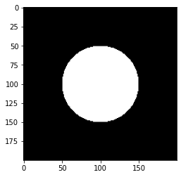
OpenCV
import numpy as np
import cv2 # opencv

im = cv2.imread('people.jpg')

type(im) # opencv로 불러올 때도 im객체가 ndarray이기 때문에 mutable이다
# numpy.ndarray

# im객체가 rectangel이라는 함수를 사용하면 결과가 누적된다 (mutable)
im_r = cv2.rectangle(im, (100,100), (250,250), (255,0,0), 10) # 두번째 인자는 직사각형에서 왼쪽 위 좌표, 오른쪽 아래 좌표 / 세번째 인자는 RGB / 네번째 인자는 테두리 크기
plt.figure(figsize=(6,6))
plt.imshow(im_r);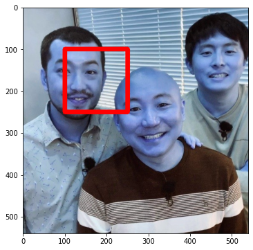
텍스트 그리기
opencv에서는 font변경이 한정적이기 때문에 기본적으로 한글 사용 불가하다
opencv를 font를 바꾸고 나서 compile하면 한글 사용할 수 있다
beatmap형태를 지원한다
im = cv2.imread('people.jpg')
cv2.putText(im, 'moon', (200,100), 1, 6, (255,0,0), 2)  # 이미지 / 텍스트 / 위치 / 폰트 / 폰트크기 / RGB / 두께

for i in dir(cv2):
  if 'FONT' in i:
    print(i, getattr(cv2, i))
plt.figure(figsize=(6,6))
plt.imshow(im)im = cv2.imread('people.jpg')
cv2.putText(im, '한글', (200,100), 1, 6, (255,0,0), 2)
plt.figure(figsize=(6,6))
plt.imshow(im)이미지 합성
주의 해야할 연산 두 가지
1. saturated : 255넘을 때 나머지 무시 => cv2.add
2. modular : % 255넘을 때 255나눈 나머지 => np.add
im1 = cv2.imread('people.jpg')
im2 = cv2.imread('apple.jpg')

cv2.addWeighted(im1, 0.7, im2, 0.3, 0) # im1의 불투명도를 70% im2의 불투명도를 30% / 두 개 이미지 shape이 같아야 한다
# error: OpenCV(4.1.2) /io/opencv/modules/core/src/arithm.cpp:663: error: (-209:Sizes of input arguments do not match) The operation is neither 'array op array' (where arrays have the same size and the same number of channels), nor 'array op scalar', nor 'scalar op array' in function 'arithm_op'
im1.shape, im2.shape
((540, 540, 3), (1000, 816, 3))
im2[:540,:540].shape
im2 = im2[250:790,150:690]
blend = cv2.addWeighted(im1, 0.7, im2, 0.3, 0) # 합성 이미지 / blending => 크기와 채널이 같아야 한다 / 두 이미지를 합 할때 가중치를 두고 연산한다 (가중합)
plt.imshow(blend)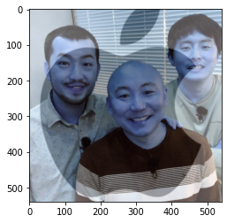
Bitwise 연산
a = 20
bin(a)
# '0b10100'

a.bit_length()
# 5

a = 20
b = 21

# 10100
# 10101
#   ↓
# 10100
a&b # bitwise and 연산 / 둘 다 1일 때 1, 둘 중 하나라도 0이면 0
# 20

# 10100
# 10101
#   ↓
# 10101
a|b # bitwise or 연산 / 둘 중 하나라도 1이면 1, 둘 다 0이면 0
# 21

bin(a),bin(b)
# ('0b10100', '0b10101')

a >> 2  # 두 칸 뒤로 / 10100 => 00101
# 5

a << 2 # 두 칸 앞으로 / 10100 => 1010000
# 80
이미지에서 bitwise 연산
im1 = cv2.imread('people.jpg', 0)
im2 = cv2.imread('apple.jpg', 0)

im2 = im2[250:790,150:690]
t=cv2.bitwise_and(im1, im2)

plt.imshow(t, cmap='gray') # masking
Opencv masking
im1 = np.zeros((200,200))
im2 = np.zeros((200,200))

h1,w1 = rectangle((40,40),(160,160))
h2,w2 = circle(100,100,50)

im1[h1,w1] = 255
im2[h2,w2] = 255
plt.imshow(cv2.bitwise_and(im1,im2), cmap='gray');
plt.imshow(cv2.bitwise_or(im1,im2), cmap='gray');
plt.imshow(cv2.bitwise_xor(im1,im2), cmap='gray');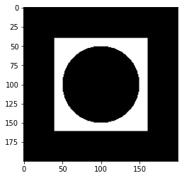
PIL
from PIL import Image, ImageDraw, ImageDraw2, ImageOps
import PIL

im_pil = Image.open('people.jpg')

type(im_pil)
# PIL.JpegImagePlugin.JpegImageFile

dir(PIL.JpegImagePlugin.JpegImageFile)
PIL.JpegImagePlugin.JpegImageFile.__class__
# type

im_pil
type(ImageDraw.ImageDraw) # Class
# type

type(ImageDraw.Draw) # function
# function

draw = ImageDraw.ImageDraw(im_pil) # composition 방식
draw2 = ImageDraw.Draw(im_pil) # function 방식 / function 방식이지만 return이 instacne이기 때문에 헷갈려서 대문자로 만들었다

draw.rectangle(((0,0),(100,100))) # mutable 방식
draw2.rectangle(((100,100),(200,200)))

im_pil
type(ImageOps)
# module

ImageOps.expand(im_pil, 20) # composition 함수 / im_pil이라는 인스턴스를 인자로 넣고 사용하기 때문에 composition 방식이다 / 결과가
텍스트 그리기
im_pil = Image.open('people.jpg')
from PIL import ImageFont
draw = ImageDraw.ImageDraw(im_pil)
draw2 = ImageDraw.Draw(im_pil)
draw.text((120,100),'Chim') # mutable 방식
im_pil
draw.text((100,120),'한글') # 기본적인 방식에서는 한글 지원 안한다

UnicodeEncodeError: 'latin-1' codec can't encode characters in position 0-1: ordinal not in range(256)
!sudo apt-get install -y fonts-nanum # colab에서 사용시 폰트를 다운 받아야 한다
!sudo fc-cache -fv
!rm ~/.cache/matplotlib -rffont = ImageFont.truetype('NanumBarunGothic', 35) # PIL은 truetype으로 깔끔하게 나온다
draw.text((240,170),'주호민', font=font, fill='pink')
im_pil
'Computer_Science > Visual Intelligence' 카테고리의 다른 글
| 9일차 - 영상 데이터 기계학습 활용 (0) | 2021.09.21 |
|---|---|
| 9일차 image 처리 (4) (0) | 2021.09.21 |
| 7일차 - Image 처리 (2) (0) | 2021.09.21 |
| 6일차 - Image 처리 (1) (0) | 2021.09.21 |
| 5일차 - 영상 데이터 처리를 위한 Array 프로그래밍 + image 처리 (0) | 2021.09.18 |