728x90
반응형
picher_stats_2017.csv
0.01MB
batter_stats_2017.csv
0.02MB
# 프로야구 연봉 예측
import pandas as pd
import numpy as np
import matplotlib.pyplot as plt
picher_file_path = 'picher_stats_2017.csv'
batter_file_path = 'batter_stats_2017.csv'
picher = pd.read_csv(picher_file_path)
batter = pd.read_csv(batter_file_path)
batter.columns

Index(['선수명', '팀명', '경기', '타석', '타수', '안타', '홈런', '득점', '타점', '볼넷', '삼진', '도루',
       'BABIP', '타율', '출루율', '장타율', 'OPS', 'wOBA', 'WAR', '연봉(2018)',
       '연봉(2017)'],
      dtype='object')
pi_fea_df = picher[['승','패','세','홀드','블론','경기','선발','이닝','삼진/9',
                    '볼넷/9','홈런/9','BABIP','LOB%','ERA','RA9-WAR','FIP','kFIP','WAR','연봉(2018)','연봉(2017)']]
pi_fea_df.info()

<class 'pandas.core.frame.DataFrame'>
RangeIndex: 152 entries, 0 to 151
Data columns (total 20 columns):
 #   Column    Non-Null Count  Dtype
---  ------    --------------  -----
 0   승         152 non-null    int64
 1   패         152 non-null    int64
 2   세         152 non-null    int64
 3   홀드        152 non-null    int64
 4   블론        152 non-null    int64
 5   경기        152 non-null    int64
 6   선발        152 non-null    int64
 7   이닝        152 non-null    float64
 8   삼진/9      152 non-null    float64
 9   볼넷/9      152 non-null    float64
 10  홈런/9      152 non-null    float64
 11  BABIP     152 non-null    float64
 12  LOB%      152 non-null    float64
 13  ERA       152 non-null    float64
 14  RA9-WAR   152 non-null    float64
 15  FIP       152 non-null    float64
 16  kFIP      152 non-null    float64
 17  WAR       152 non-null    float64
 18  연봉(2018)  152 non-null    int64
 19  연봉(2017)  152 non-null    int64
dtypes: float64(11), int64(9)
memory usage: 23.9 KB
picher = picher.rename(columns = {'연봉(2018)':'y'})

team_encoding = pd.get_dummies(picher['팀명'])
team_encoding.head()

KIA	KT	LG	NC	SK	두산	롯데	삼성	한화
0	0	0	0	0	1	0	0	0	0
1	0	0	1	0	0	0	0	0	0
2	1	0	0	0	0	0	0	0	0
3	0	0	1	0	0	0	0	0	0
4	0	0	0	0	0	0	1	0	0
picher = pd.concat([picher, team_encoding], axis=1)
picher.head()

	선수명	팀명	승	패	세	홀드	블론	경기	선발	이닝	...	연봉(2017)	KIA	KT	LG	NC	SK	두산	롯데	삼성	한화
0	켈리	SK	16	7	0	0	0	30	30	190.0	...	85000	0	0	0	0	1	0	0	0	0
1	소사	LG	11	11	1	0	0	30	29	185.1	...	50000	0	0	1	0	0	0	0	0	0
2	양현종	KIA	20	6	0	0	0	31	31	193.1	...	150000	1	0	0	0	0	0	0	0	0
3	차우찬	LG	10	7	0	0	0	28	28	175.2	...	100000	0	0	1	0	0	0	0	0	0
4	레일리	롯데	13	7	0	0	0	30	30	187.1	...	85000	0	0	0	0	0	0	1	0	0
5 rows × 31 columns
picher = picher.drop('팀명', axis=1)

x = picher[picher.columns.difference({'선수명','y'})]
y = picher['y']
from sklearn import preprocessing as pp
x = pp.StandardScaler().fit(x).transform(x)
pd.options.mode.chained_assignment = None # 과학적표기방법 안씀
# 정규화 함수
def standard_scaling(df, scale_columns) :
    for col in scale_columns :
        s_mean = df[col].mean()
        s_std = df[col].std()
        df[col] =  df[col].apply(lambda x : (x - s_mean)/s_std)
    return df
pi_fea_df = picher[['승','패','세','홀드','블론','경기','선발','이닝','삼진/9',
                    '볼넷/9','홈런/9','BABIP','LOB%','ERA','RA9-WAR','FIP','kFIP','WAR','연봉(2017)']]
pi_fea_df.info()

<class 'pandas.core.frame.DataFrame'>
RangeIndex: 152 entries, 0 to 151
Data columns (total 19 columns):
 #   Column    Non-Null Count  Dtype
---  ------    --------------  -----
 0   승         152 non-null    float64
 1   패         152 non-null    float64
 2   세         152 non-null    float64
 3   홀드        152 non-null    float64
 4   블론        152 non-null    float64
 5   경기        152 non-null    float64
 6   선발        152 non-null    float64
 7   이닝        152 non-null    float64
 8   삼진/9      152 non-null    float64
 9   볼넷/9      152 non-null    float64
 10  홈런/9      152 non-null    float64
 11  BABIP     152 non-null    float64
 12  LOB%      152 non-null    float64
 13  ERA       152 non-null    float64
 14  RA9-WAR   152 non-null    float64
 15  FIP       152 non-null    float64
 16  kFIP      152 non-null    float64
 17  WAR       152 non-null    float64
 18  연봉(2017)  152 non-null    int64
dtypes: float64(18), int64(1)
memory usage: 22.7 KB
picher_df = standard_scaling(picher,pi_fea_df )
# 정규화된 x
x = picher[picher_df.columns.difference({'선수명','y'})]
x.head()

	BABIP	ERA	FIP	KIA	KT	LG	LOB%	NC	RA9-WAR	SK	...	삼진/9	선발	세	승	연봉(2017)	이닝	패	한화	홀드	홈런/9
0	0.016783	-0.587056	-0.971030	0	0	0	0.446615	0	3.174630	1	...	0.672099	2.452068	-0.306452	3.313623	2.734705	2.645175	1.227145	0	-0.585705	-0.442382
1	-0.241686	-0.519855	-1.061888	0	0	1	-0.122764	0	3.114968	0	...	0.134531	2.349505	-0.098502	2.019505	1.337303	2.547755	2.504721	0	-0.585705	-0.668521
2	-0.095595	-0.625456	-0.837415	1	0	0	0.308584	0	2.973948	0	...	0.109775	2.554632	-0.306452	4.348918	5.329881	2.706808	0.907751	0	-0.585705	-0.412886
3	-0.477680	-0.627856	-0.698455	0	0	1	0.558765	0	2.740722	0	...	0.350266	2.246942	-0.306452	1.760682	3.333592	2.350927	1.227145	0	-0.585705	-0.186746
4	-0.196735	-0.539055	-0.612941	0	0	0	0.481122	0	2.751570	0	...	0.155751	2.452068	-0.306452	2.537153	2.734705	2.587518	1.227145	0	-0.585705	-0.294900
5 rows × 28 columns
from sklearn.model_selection import train_test_split
x_train, x_test, y_train, y_test = train_test_split(x, y, test_size=0.2, random_state=19)

picher.info()

<class 'pandas.core.frame.DataFrame'>
RangeIndex: 152 entries, 0 to 151
Data columns (total 30 columns):
 #   Column    Non-Null Count  Dtype
---  ------    --------------  -----
 0   선수명       152 non-null    object
 1   승         152 non-null    float64
 2   패         152 non-null    float64
 3   세         152 non-null    float64
 4   홀드        152 non-null    float64
 5   블론        152 non-null    float64
 6   경기        152 non-null    float64
 7   선발        152 non-null    float64
 8   이닝        152 non-null    float64
 9   삼진/9      152 non-null    float64
 10  볼넷/9      152 non-null    float64
 11  홈런/9      152 non-null    float64
 12  BABIP     152 non-null    float64
 13  LOB%      152 non-null    float64
 14  ERA       152 non-null    float64
 15  RA9-WAR   152 non-null    float64
 16  FIP       152 non-null    float64
 17  kFIP      152 non-null    float64
 18  WAR       152 non-null    float64
 19  y         152 non-null    int64
 20  연봉(2017)  152 non-null    float64
 21  KIA       152 non-null    uint8
 22  KT        152 non-null    uint8
 23  LG        152 non-null    uint8
 24  NC        152 non-null    uint8
 25  SK        152 non-null    uint8
 26  두산        152 non-null    uint8
 27  롯데        152 non-null    uint8
 28  삼성        152 non-null    uint8
 29  한화        152 non-null    uint8
dtypes: float64(19), int64(1), object(1), uint8(9)
memory usage: 26.4+ KB
# ols
import statsmodels.api as sm

x_train = sm.add_constant(x_train)
model = sm.OLS(y_train, x_train).fit()
model.summary()

OLS Regression Results
Dep. Variable:	y	R-squared:	0.928
Model:	OLS	Adj. R-squared:	0.907
Method:	Least Squares	F-statistic:	44.19
Date:	Tue, 20 Jul 2021	Prob (F-statistic):	7.70e-42
Time:	10:11:19	Log-Likelihood:	-1247.8
No. Observations:	121	AIC:	2552.
Df Residuals:	93	BIC:	2630.
Df Model:	27
Covariance Type:	nonrobust
coef	std err	t	P>|t|	[0.025	0.975]
const	1.872e+04	775.412	24.136	0.000	1.72e+04	2.03e+04
x1	-1476.1375	1289.136	-1.145	0.255	-4036.106	1083.831
x2	-415.3144	2314.750	-0.179	0.858	-5011.949	4181.320
x3	-9.383e+04	9.4e+04	-0.998	0.321	-2.8e+05	9.28e+04
x4	-485.0276	671.883	-0.722	0.472	-1819.254	849.199
x5	498.2459	695.803	0.716	0.476	-883.480	1879.972
x6	-262.5237	769.196	-0.341	0.734	-1789.995	1264.948
x7	-1371.0060	1559.650	-0.879	0.382	-4468.162	1726.150
x8	-164.7210	760.933	-0.216	0.829	-1675.784	1346.342
x9	3946.0617	2921.829	1.351	0.180	-1856.111	9748.235
x10	269.1233	721.020	0.373	0.710	-1162.679	1700.926
x11	1.024e+04	2523.966	4.057	0.000	5226.545	1.53e+04
x12	7.742e+04	7.93e+04	0.977	0.331	-8e+04	2.35e+05
x13	-2426.3684	2943.799	-0.824	0.412	-8272.169	3419.432
x14	-285.5830	781.560	-0.365	0.716	-1837.606	1266.440
x15	111.1761	758.548	0.147	0.884	-1395.150	1617.502
x16	7587.0753	6254.661	1.213	0.228	-4833.443	2e+04
x17	1266.8570	1238.036	1.023	0.309	-1191.636	3725.350
x18	-972.1837	817.114	-1.190	0.237	-2594.810	650.443
x19	5379.1903	7262.214	0.741	0.461	-9042.128	1.98e+04
x20	-4781.4961	5471.265	-0.874	0.384	-1.56e+04	6083.352
x21	-249.8717	1291.108	-0.194	0.847	-2813.757	2314.014
x22	235.2476	2207.965	0.107	0.915	-4149.333	4619.828
x23	1.907e+04	1266.567	15.055	0.000	1.66e+04	2.16e+04
x24	851.2121	6602.114	0.129	0.898	-1.23e+04	1.4e+04
x25	1297.3310	1929.556	0.672	0.503	-2534.385	5129.047
x26	1199.4709	720.099	1.666	0.099	-230.503	2629.444
x27	-931.9918	1632.526	-0.571	0.569	-4173.865	2309.882
x28	1.808e+04	1.67e+04	1.082	0.282	-1.51e+04	5.13e+04
Omnibus:	28.069	Durbin-Watson:	2.025
Prob(Omnibus):	0.000	Jarque-Bera (JB):	194.274
Skew:	-0.405	Prob(JB):	6.52e-43
Kurtosis:	9.155	Cond. No.	1.23e+16


Notes:
[1] Standard Errors assume that the covariance matrix of the errors is correctly specified.
[2] The smallest eigenvalue is 5.36e-30. This might indicate that there are
strong multicollinearity problems or that the design matrix is singular.
# r_squared 결정계수
독립변수의 변동량으로 설명되는 종속변수의 변동량
상관계수의 제곱과 가다
# adj 수정결정계수
독립변수가 많아지는 경우 결정계수값이 커질수있어, 표본의 크기와 독립변수의 수를 고려하여
다중회귀분석을 수행하는 경우
p>|t| 각피처의 검정통계량(f statistics )이 유의미한지를 나타내는 pvalue 값
p value < 0.05 이면 피처가 회귀분석에 유의미한 피처다
이분석에서는 war 연복2017 한화 3개가 0.05미만
=> 회귀분석에서 유의미한 피처들
x_train = sm.add_constant(x_train)
model = sm.OLS(y_train, x_train).fit()
model.summary()

OLS Regression Results
Dep. Variable:	y	R-squared:	0.928
Model:	OLS	Adj. R-squared:	0.907
Method:	Least Squares	F-statistic:	44.19
Date:	Tue, 20 Jul 2021	Prob (F-statistic):	7.70e-42
Time:	10:53:15	Log-Likelihood:	-1247.8
No. Observations:	121	AIC:	2552.
Df Residuals:	93	BIC:	2630.
Df Model:	27
Covariance Type:	nonrobust
coef	std err	t	P>|t|	[0.025	0.975]
const	1.678e+04	697.967	24.036	0.000	1.54e+04	1.82e+04
BABIP	-1481.0173	1293.397	-1.145	0.255	-4049.448	1087.414
ERA	-416.6874	2322.402	-0.179	0.858	-5028.517	4195.143
FIP	-9.414e+04	9.43e+04	-0.998	0.321	-2.81e+05	9.31e+04
KIA	303.1852	2222.099	0.136	0.892	-4109.462	4715.833
KT	3436.0520	2133.084	1.611	0.111	-799.831	7671.935
LG	1116.9978	2403.317	0.465	0.643	-3655.513	5889.509
LOB%	-1375.5383	1564.806	-0.879	0.382	-4482.933	1731.857
NC	1340.5004	2660.966	0.504	0.616	-3943.651	6624.652
RA9-WAR	3959.1065	2931.488	1.351	0.180	-1862.247	9780.460
SK	2762.4237	2243.540	1.231	0.221	-1692.803	7217.650
WAR	1.027e+04	2532.309	4.057	0.000	5243.823	1.53e+04
kFIP	7.767e+04	7.95e+04	0.977	0.331	-8.03e+04	2.36e+05
경기	-2434.3895	2953.530	-0.824	0.412	-8299.515	3430.736
두산	971.9293	2589.849	0.375	0.708	-4170.998	6114.857
롯데	2313.9585	2566.009	0.902	0.370	-2781.627	7409.544
볼넷/9	7612.1566	6275.338	1.213	0.228	-4849.421	2.01e+04
블론	1271.0450	1242.128	1.023	0.309	-1195.576	3737.666
삼성	-946.5092	2482.257	-0.381	0.704	-5875.780	3982.762
삼진/9	5396.9728	7286.221	0.741	0.461	-9072.019	1.99e+04
선발	-4797.3028	5489.352	-0.874	0.384	-1.57e+04	6103.463
세	-250.6977	1295.377	-0.194	0.847	-2823.059	2321.663
승	236.0253	2215.264	0.107	0.915	-4163.049	4635.100
연봉(2017)	1.913e+04	1270.754	15.055	0.000	1.66e+04	2.17e+04
이닝	854.0260	6623.940	0.129	0.898	-1.23e+04	1.4e+04
패	1301.6197	1935.935	0.672	0.503	-2542.763	5146.003
한화	5477.8879	2184.273	2.508	0.014	1140.355	9815.421
홀드	-935.0728	1637.923	-0.571	0.569	-4187.663	2317.518
홈런/9	1.814e+04	1.68e+04	1.082	0.282	-1.52e+04	5.14e+04
Omnibus:	28.069	Durbin-Watson:	2.025
Prob(Omnibus):	0.000	Jarque-Bera (JB):	194.274
Skew:	-0.405	Prob(JB):	6.52e-43
Kurtosis:	9.155	Cond. No.	3.63e+16


Notes:
[1] Standard Errors assume that the covariance matrix of the errors is correctly specified.
[2] The smallest eigenvalue is 6.04e-31. This might indicate that there are
strong multicollinearity problems or that the design matrix is singular.
plt.rcParams['figure.figsize'] = [20, 16]
plt.rc('font', family = 'Malgun Gothic')
coefs = model.params.tolist()
coefs_series = pd.Series(coefs)
x_labels = model.params.index.tolist()
ax = coefs_series.plot(kind = 'bar')
ax.set_title('feature_coef_graph')
ax.set_xlabel('x_feature')
ax.set_ylabel('coef')
ax.set_xticklabels(x_labels)

[Text(0, 0, 'const'),
 Text(1, 0, 'BABIP'),
 Text(2, 0, 'ERA'),
 Text(3, 0, 'FIP'),
 Text(4, 0, 'KIA'),
 Text(5, 0, 'KT'),
 Text(6, 0, 'LG'),
 Text(7, 0, 'LOB%'),
 Text(8, 0, 'NC'),
 Text(9, 0, 'RA9-WAR'),
 Text(10, 0, 'SK'),
 Text(11, 0, 'WAR'),
 Text(12, 0, 'kFIP'),
 Text(13, 0, '경기'),
 Text(14, 0, '두산'),
 Text(15, 0, '롯데'),
 Text(16, 0, '볼넷/9'),
 Text(17, 0, '블론'),
 Text(18, 0, '삼성'),
 Text(19, 0, '삼진/9'),
 Text(20, 0, '선발'),
 Text(21, 0, '세'),
 Text(22, 0, '승'),
 Text(23, 0, '연봉(2017)'),
 Text(24, 0, '이닝'),
 Text(25, 0, '패'),
 Text(26, 0, '한화'),
 Text(27, 0, '홀드'),
 Text(28, 0, '홈런/9')]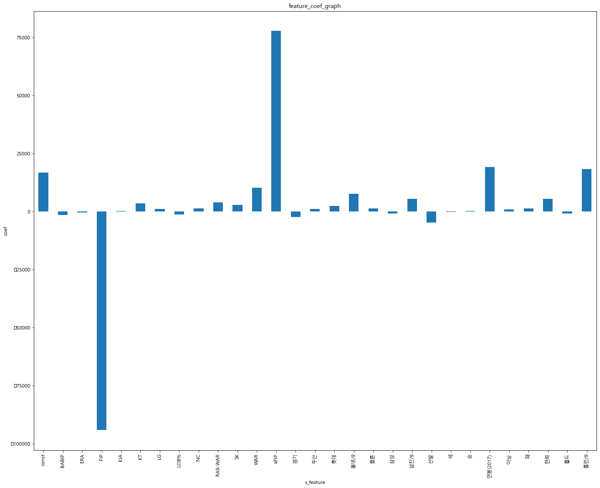
다중공선성이 높으면 상관성이 너무 높은 것
안정적인 분석을 위해서 안써야함
from statsmodels.stats.outliers_influence import variance_inflation_factor
vif = pd.DataFrame()
vif['VIF Factor'] = [variance_inflation_factor(x.values, i) for i in range(x.shape[1])]
vif['features'] = x.columns
vif.round(1)

	VIF Factor	features
0	3.2	BABIP
1	10.6	ERA
2	14238.3	FIP
3	1.1	KIA
4	1.1	KT
5	1.1	LG
6	4.3	LOB%
7	1.1	NC
8	13.6	RA9-WAR
9	1.1	SK
10	10.4	WAR
11	10264.1	kFIP
12	14.6	경기
13	1.2	두산
14	1.1	롯데
15	57.8	볼넷/9
16	3.0	블론
17	1.2	삼성
18	89.5	삼진/9
19	39.6	선발
20	3.1	세
21	8.0	승
22	2.5	연봉(2017)
23	63.8	이닝
24	5.9	패
25	1.1	한화
26	3.8	홀드
27	425.6	홈런/9
변수간 상관관계가 높아서 분석에 부정적인 영향을 미침
vif 평가 : 분산팽창요인
보통 10~15 정도를 넘으면 다중공선성에 문제가 있다고 판단
홈런, 이닝, 선발, 삼진, 볼넷, 경기, kfip,fip
특히 이둘은 너무 유사해서 상승효과가 생김, 그래서 하나는 빼버려야함
1. vif 계수 높은 피처 제거, 유사피처중 한개만 제거
2. 다시모델을 실행해서 공선성 검증
3. 분석결과에서 p-value값이 유의미한 피처들을 선정
# 적절한 피처를 선정해서 다시 학습하기
# 피처간 상관계수를 그래프로 작성
scale_columns = ['승','패','세','홀드','블론','경기','선발','이닝','삼진/9',
                    '볼넷/9','홈런/9','BABIP','LOB%','ERA','RA9-WAR','FIP','kFIP','WAR','연봉(2017)']
picher_df.info()
<class 'pandas.core.frame.DataFrame'>
RangeIndex: 152 entries, 0 to 151
Data columns (total 30 columns):
 #   Column    Non-Null Count  Dtype
---  ------    --------------  -----
 0   선수명       152 non-null    object
 1   승         152 non-null    float64
 2   패         152 non-null    float64
 3   세         152 non-null    float64
 4   홀드        152 non-null    float64
 5   블론        152 non-null    float64
 6   경기        152 non-null    float64
 7   선발        152 non-null    float64
 8   이닝        152 non-null    float64
 9   삼진/9      152 non-null    float64
 10  볼넷/9      152 non-null    float64
 11  홈런/9      152 non-null    float64
 12  BABIP     152 non-null    float64
 13  LOB%      152 non-null    float64
 14  ERA       152 non-null    float64
 15  RA9-WAR   152 non-null    float64
 16  FIP       152 non-null    float64
 17  kFIP      152 non-null    float64
 18  WAR       152 non-null    float64
 19  y         152 non-null    int64
 20  연봉(2017)  152 non-null    float64
 21  KIA       152 non-null    uint8
 22  KT        152 non-null    uint8
 23  LG        152 non-null    uint8
 24  NC        152 non-null    uint8
 25  SK        152 non-null    uint8
 26  두산        152 non-null    uint8
 27  롯데        152 non-null    uint8
 28  삼성        152 non-null    uint8
 29  한화        152 non-null    uint8
dtypes: float64(19), int64(1), object(1), uint8(9)
memory usage: 26.4+ KB
corr = picher_df[scale_columns].corr(method='pearson')
corr

	승	패	세	홀드	블론	경기	선발	이닝	삼진/9	볼넷/9	홈런/9	BABIP	LOB%	ERA	RA9-WAR	FIP	kFIP	WAR	연봉(2017)
승	1.000000	0.710749	0.053747	0.092872	0.105281	0.397074	0.773560	0.906093	0.078377	-0.404710	-0.116147	-0.171111	0.131178	-0.271086	0.851350	-0.303133	-0.314159	0.821420	0.629710
패	0.710749	1.000000	0.066256	0.098617	0.121283	0.343147	0.771395	0.829018	0.031755	-0.386313	-0.064467	-0.133354	-0.020994	-0.188036	0.595989	-0.233416	-0.238688	0.625641	0.429227
세	0.053747	0.066256	1.000000	0.112716	0.605229	0.434290	-0.177069	0.020278	0.170436	-0.131394	-0.073111	-0.089212	0.167557	-0.150348	0.167669	-0.199746	-0.225259	0.084151	0.262664
홀드	0.092872	0.098617	0.112716	1.000000	0.490076	0.715527	-0.285204	0.024631	0.186790	-0.146806	-0.076475	-0.104307	0.048123	-0.155712	0.003526	-0.211515	-0.237353	-0.038613	-0.001213
블론	0.105281	0.121283	0.605229	0.490076	1.000000	0.630526	-0.264160	0.014176	0.188423	-0.137019	-0.064804	-0.112480	0.100633	-0.160761	0.008766	-0.209014	-0.237815	-0.058213	0.146584
경기	0.397074	0.343147	0.434290	0.715527	0.630526	1.000000	-0.037443	0.376378	0.192487	-0.364293	-0.113545	-0.241608	0.105762	-0.320177	0.281595	-0.345351	-0.373777	0.197836	0.225357
선발	0.773560	0.771395	-0.177069	-0.285204	-0.264160	-0.037443	1.000000	0.894018	-0.055364	-0.312935	-0.058120	-0.098909	0.041819	-0.157775	0.742258	-0.151040	-0.142685	0.758846	0.488559
이닝	0.906093	0.829018	0.020278	0.024631	0.014176	0.376378	0.894018	1.000000	0.037343	-0.451101	-0.107063	-0.191514	0.103369	-0.285392	0.853354	-0.296768	-0.302288	0.832609	0.586874
삼진/9	0.078377	0.031755	0.170436	0.186790	0.188423	0.192487	-0.055364	0.037343	1.000000	0.109345	0.216017	0.457523	-0.071284	0.256840	0.102963	-0.154857	-0.317594	0.151791	0.104948
볼넷/9	-0.404710	-0.386313	-0.131394	-0.146806	-0.137019	-0.364293	-0.312935	-0.451101	0.109345	1.000000	0.302251	0.276009	-0.150837	0.521039	-0.398586	0.629833	0.605008	-0.394131	-0.332379
홈런/9	-0.116147	-0.064467	-0.073111	-0.076475	-0.064804	-0.113545	-0.058120	-0.107063	0.216017	0.302251	1.000000	0.362614	-0.274543	0.629912	-0.187210	0.831042	0.743623	-0.205014	-0.100896
BABIP	-0.171111	-0.133354	-0.089212	-0.104307	-0.112480	-0.241608	-0.098909	-0.191514	0.457523	0.276009	0.362614	1.000000	-0.505478	0.733109	-0.187058	0.251126	0.166910	-0.082995	-0.088754
LOB%	0.131178	-0.020994	0.167557	0.048123	0.100633	0.105762	0.041819	0.103369	-0.071284	-0.150837	-0.274543	-0.505478	1.000000	-0.720091	0.286893	-0.288050	-0.269536	0.144191	0.110424
ERA	-0.271086	-0.188036	-0.150348	-0.155712	-0.160761	-0.320177	-0.157775	-0.285392	0.256840	0.521039	0.629912	0.733109	-0.720091	1.000000	-0.335584	0.648004	0.582057	-0.261508	-0.203305
RA9-WAR	0.851350	0.595989	0.167669	0.003526	0.008766	0.281595	0.742258	0.853354	0.102963	-0.398586	-0.187210	-0.187058	0.286893	-0.335584	1.000000	-0.366308	-0.377679	0.917299	0.643375
FIP	-0.303133	-0.233416	-0.199746	-0.211515	-0.209014	-0.345351	-0.151040	-0.296768	-0.154857	0.629833	0.831042	0.251126	-0.288050	0.648004	-0.366308	1.000000	0.984924	-0.391414	-0.268005
kFIP	-0.314159	-0.238688	-0.225259	-0.237353	-0.237815	-0.373777	-0.142685	-0.302288	-0.317594	0.605008	0.743623	0.166910	-0.269536	0.582057	-0.377679	0.984924	1.000000	-0.408283	-0.282666
WAR	0.821420	0.625641	0.084151	-0.038613	-0.058213	0.197836	0.758846	0.832609	0.151791	-0.394131	-0.205014	-0.082995	0.144191	-0.261508	0.917299	-0.391414	-0.408283	1.000000	0.675794
연봉(2017)	0.629710	0.429227	0.262664	-0.001213	0.146584	0.225357	0.488559	0.586874	0.104948	-0.332379	-0.100896	-0.088754	0.110424	-0.203305	0.643375	-0.268005	-0.282666	0.675794	1.000000
# 히트맵 시각화
import seaborn as sns
show_cols = ['win', 'lose','save','hold','blon','match','start','inning','strike3',
            'ball4','homerun','BABIP','LOB','ERA','RA9-WAR','FIP','kFIP','WAR','2017']
plt.rc('font', family = 'Nanum Gothic')
sns.set(font_scale=0.8)
hm = sns.heatmap(corr.values,
                cbar = True,
                annot = True,
                square = True,
                fmt = '.2f',
                annot_kws={'size':15},
                yticklabels = show_cols,
                xticklabels = show_cols)
plt.tight_layout()
plt.show()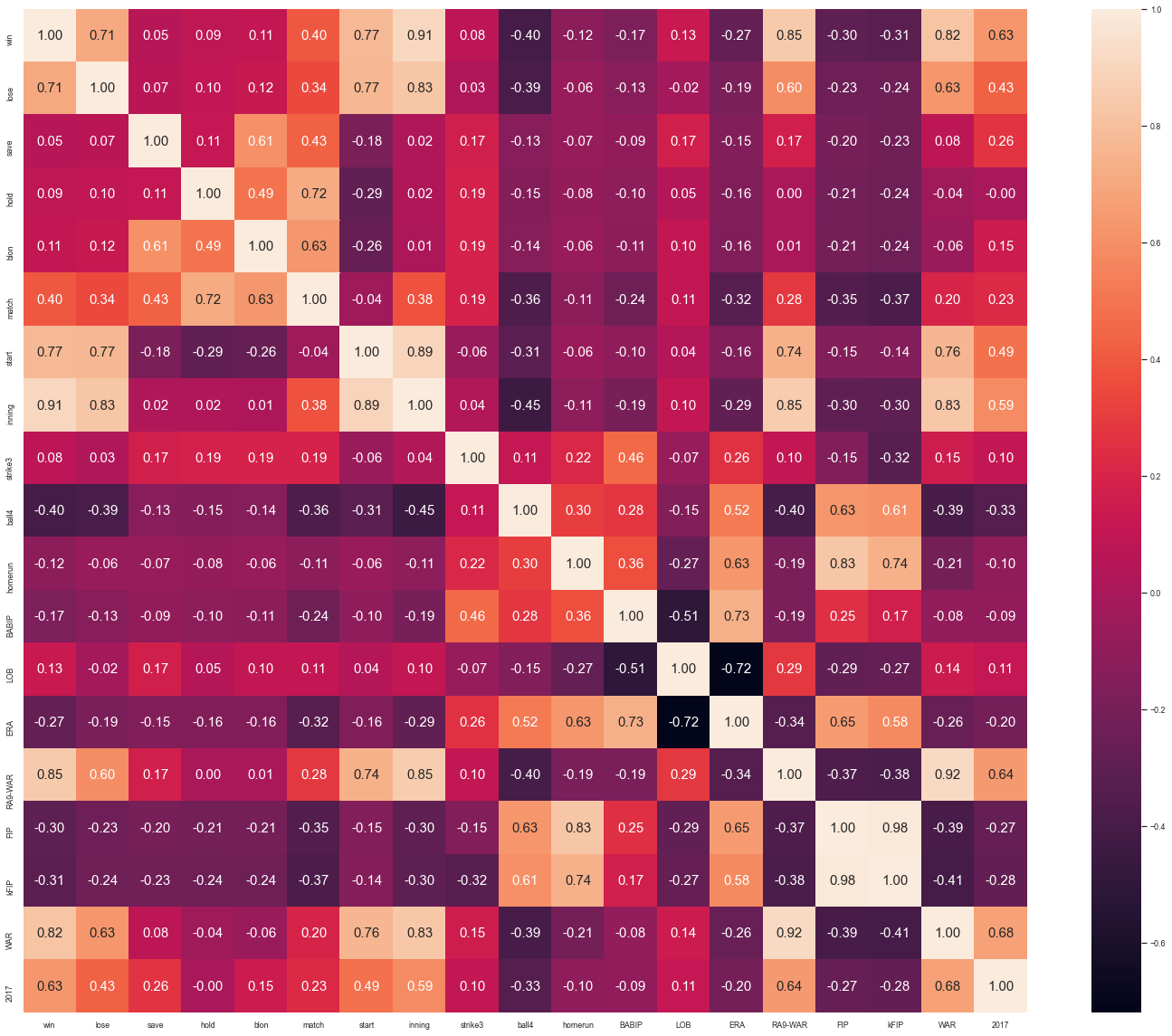
x = picher_df[['FIP','WAR','볼넷/9','삼진/9','연봉(2017)']]
y = picher_df['y']
from sklearn.model_selection import train_test_split
x_train, x_test, y_train, y_test = train_test_split(x, y, test_size=0.2, random_state=19)
# 모델학습하기
from sklearn.linear_model import LinearRegression
lr = LinearRegression()
model = lr.fit(x_train, y_train)
# r2
print(model.score(x_train, y_train))
print(model.score(x_test, y_test))

# 0.9150591192570362
# 0.9038759653889865
# rmse 평가
# mse 평균제곱오차
from math import sqrt
from sklearn.metrics import mean_squared_error
y_pred = lr.predict(x_train)
print(sqrt(mean_squared_error(y_train, y_pred)))
y_pred = lr.predict(x_test)
print(sqrt(mean_squared_error(y_test, y_pred)))

# 7893.462873347693
# 13141.86606359108
# 피처별 vif 공분산
from statsmodels.stats.outliers_influence import variance_inflation_factor
x = picher_df[['FIP','WAR','볼넷/9','삼진/9','연봉(2017)']]
vif = pd.DataFrame()
vif['VIF Factor'] = [variance_inflation_factor(x.values, i) for i in range(x.shape[1])]
vif['features'] = x.columns
vif.round(1)


	VIF Factor	features
0	1.9	FIP
1	2.1	WAR
2	1.9	볼넷/9
3	1.1	삼진/9
4	1.9	연봉(2017)
# 시각화\ 비교
# 모든 데이터 검증
# lr 학습이 완료된 객체
x = picher_df[['FIP','WAR','볼넷/9','삼진/9','연봉(2017)']]
predict_2018_salary = lr.predict(x)
predict_2018_salary[:5]
picher_df['예측연봉(2018)'] = pd.Series(predict_2018_salary)
picher = pd.read_csv(picher_file_path)
picher = picher[['선수명','연봉(2017)']]
# 2018년 연봉 내림차순
result_df = picher_df.sort_values(by=['y'], ascending = False)
# 연봉2017 삭제, 정규화된 데이터, 실제데이터가 아님
result_df.drop(['연봉(2017)'], axis=1, inplace=True, errors='ignore')
# 연봉 2017의 실제데이터로 컬럼 변경
result_df = result_df.merge(picher, on=['선수명'], how='left')
result_df = result_df[['선수명', 'y','예측연봉(2018)','연봉(2017)']]
result_df.columns = ['선수명','실제연봉(2018)','예측연봉(2018)','작년연봉(2017)']
result_df
	선수명	실제연봉(2018)	예측연봉(2018)	작년연봉(2017)
0	양현종	230000	163930.148696	150000
1	켈리	140000	120122.822204	85000
2	소사	120000	88127.019455	50000
3	정우람	120000	108489.464585	120000
4	레일리	111000	102253.697589	85000
...	...	...	...	...
147	장지훈	2800	249.850641	2700
148	차재용	2800	900.811527	2800
149	성영훈	2700	5003.619609	2700
150	정동윤	2700	2686.350884	2700
151	장민익	2700	3543.781665	2700
152 rows × 4 columns
result_df = result_df.iloc[:10,:]
plt.rc('font', family = 'Malgun Gothic')
result_df.plot(x='선수명', y=['작년연봉(2017)','예측연봉(2018)','실제연봉(2018)'], kind='bar')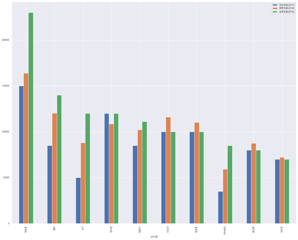
# 2017연봉과 2018년 연봉이 다른 선수들만
result_df = result_df[result_df['작년연봉(2017)'] != result_df['예측연봉(2018)']]
result_df.head()
	선수명	실제연봉(2018)	예측연봉(2018)	작년연봉(2017)
0	양현종	230000	163930.148696	150000
1	켈리	140000	120122.822204	85000
2	소사	120000	88127.019455	50000
3	정우람	120000	108489.464585	120000
4	레일리	111000	102253.697589	85000
result_df = result_df.reset_index()
result_df.head()

	index	선수명	실제연봉(2018)	예측연봉(2018)	작년연봉(2017)
0	0	양현종	230000	163930.148696	150000
1	1	켈리	140000	120122.822204	85000
2	2	소사	120000	88127.019455	50000
3	3	정우람	120000	108489.464585	120000
4	4	레일리	111000	102253.697589	85000
result_df = result_df.iloc[:10, :]
result_df.plot(x='선수명', y=['작년연봉(2017)','예측연봉(2018)','실제연봉(2018)'],kind = 'bar')
반응형
'Data_Science > Data_Analysis_Py' 카테고리의 다른 글
| 29. 비트코인 시계열 분석 || prophet (0) | 2021.11.24 |
|---|---|
| 28. 비트코인 가격 시계열 분석 || Arima, fbProphet (0) | 2021.11.24 |
| 26. 서울 중학교 졸업자 분석 || dbscan, folium (0) | 2021.11.24 |
| 25. 판매 데이터 분석 || kmeans (0) | 2021.11.24 |
| 24. 위스콘신 유방안데이터 분석 || DT (0) | 2021.11.24 |