728x90
반응형
import numpy as np
import pandas as pd
import matplotlib.pyplot as plt
from fbprophet import Prophet
file_path = 'market-price.csv'
bitcoin_df = pd.read_csv(file_path, names = ['ds', 'y'], header=0)
# 상한가 설정
bitcoin_df['cap'] = 20000
# 하한가 설정
# bitcoin_df['floor'] = 2000
# growth = logistic  상한설정시 추가, 비선형방식으로 분석
prophet = Prophet(seasonality_mode = 'multiplicative',
                  growth = 'logistic', # 상하한가 설정할때 , 비선형방식
                 yearly_seasonality = True, # 연별
                 weekly_seasonality = True, # 주별
                 daily_seasonality = True, # 일별
                 changepoint_prior_scale = 0.5) # 과적합 방지 0.5만큼 만 분석
prophet.fit(bitcoin_df) # 학습하기
bitcoin_df.head()
ds y cap
0 2017-08-27 00:00:00 4354.308333 20000
1 2017-08-28 00:00:00 4391.673517 20000
2 2017-08-29 00:00:00 4607.985450 20000
3 2017-08-30 00:00:00 4594.987850 20000
4 2017-08-31 00:00:00 4748.255000 20000
import numpy as np
import pandas as pd
import matplotlib.pyplot as plt
from fbprophet import Prophet
file_path = 'market-price.csv'
bitcoin_df = pd.read_csv(file_path, names = ['ds', 'y'], header=0)
# 상한가 설정
bitcoin_df['cap'] = 20000
# 하한가 설정
# bitcoin_df['floor'] = 2000
# growth = logistic  상한설정시 추가, 비선형방식으로 분석
prophet = Prophet(seasonality_mode = 'multiplicative',
                  growth = 'logistic', # 상하한가 설정할때 , 비선형방식
                 yearly_seasonality = True, # 연별
                 weekly_seasonality = True, # 주별
                 daily_seasonality = True, # 일별
                 changepoint_prior_scale = 0.5) # 과적합 방지 0.5만큼 만 분석
(
    growth='linear',
    changepoints=None,
    n_changepoints=25,
    changepoint_range=0.8,
    yearly_seasonality='auto',
    weekly_seasonality='auto',
    daily_seasonality='auto',
    holidays=None,
    seasonality_mode='additive',
    seasonality_prior_scale=10.0,
    holidays_prior_scale=10.0,
    changepoint_prior_scale=0.05,
    mcmc_samples=0,
    interval_width=0.8,
    uncertainty_samples=1000,
    stan_backend=None,
)
# 5일 앞을 예측하기
future_data = prophet.make_future_dataframe(periods=5, freq='d')
# 상한가 설정
future_data['cap'] = 20000
# future_data['floor'] = 2000
# 예측
forecast_data = prophet.predict(future_data)
forecast_data

	ds	trend	cap	yhat_lower	yhat_upper	trend_lower	trend_upper	daily	daily_lower	daily_upper	...	weekly	weekly_lower	weekly_upper	yearly	yearly_lower	yearly_upper	additive_terms	additive_terms_lower	additive_terms_upper	yhat
0	2017-08-27	5621.085431	20000	4008.821488	5757.019304	5621.085431	5621.085431	0.311474	0.311474	0.311474	...	0.002289	0.002289	0.002289	-0.440095	-0.440095	-0.440095	0.0	0.0	0.0	4910.962354
1	2017-08-28	5626.023045	20000	3955.585468	5723.896533	5626.023045	5626.023045	0.311474	0.311474	0.311474	...	-0.000562	-0.000562	-0.000562	-0.449330	-0.449330	-0.449330	0.0	0.0	0.0	4847.280361
2	2017-08-29	5630.963297	20000	3911.998721	5680.326522	5630.963297	5630.963297	0.311474	0.311474	0.311474	...	-0.000493	-0.000493	-0.000493	-0.459435	-0.459435	-0.459435	0.0	0.0	0.0	4795.023355
3	2017-08-30	5635.906186	20000	3875.520852	5590.533721	5635.906186	5635.906186	0.311474	0.311474	0.311474	...	-0.007356	-0.007356	-0.007356	-0.470318	-0.470318	-0.470318	0.0	0.0	0.0	4699.215406
4	2017-08-31	5640.851711	20000	3810.130956	5423.302109	5640.851711	5640.851711	0.311474	0.311474	0.311474	...	-0.005606	-0.005606	-0.005606	-0.481860	-0.481860	-0.481860	0.0	0.0	0.0	4648.105600
...	...	...	...	...	...	...	...	...	...	...	...	...	...	...	...	...	...	...	...	...	...
365	2018-08-27	7108.210766	20000	5313.384266	7048.183238	7108.210766	7108.210766	0.311474	0.311474	0.311474	...	-0.000562	-0.000562	-0.000562	-0.437930	-0.437930	-0.437930	0.0	0.0	0.0	6205.334670
366	2018-08-28	7111.966217	20000	5257.614559	7014.891617	7111.966217	7111.966217	0.311474	0.311474	0.311474	...	-0.000493	-0.000493	-0.000493	-0.446936	-0.446936	-0.446936	0.0	0.0	0.0	6145.052289
367	2018-08-29	7115.722558	20000	5183.980838	6862.843499	7115.722558	7115.722558	0.311474	0.311474	0.311474	...	-0.007356	-0.007356	-0.007356	-0.456831	-0.456831	-0.456831	0.0	0.0	0.0	6029.053882
368	2018-08-30	7119.479786	20000	5142.817816	6755.514784	7119.464525	7119.496318	0.311474	0.311474	0.311474	...	-0.005606	-0.005606	-0.005606	-0.467530	-0.467530	-0.467530	0.0	0.0	0.0	5968.527240
369	2018-08-31	7123.237902	20000	5101.560913	6845.461477	7123.183774	7123.294421	0.311474	0.311474	0.311474	...	0.000310	0.000310	0.000310	-0.478920	-0.478920	-0.478920	0.0	0.0	0.0	5932.681373
370 rows × 23 columns
# 그래프로 작성
fig = prophet.plot(forecast_data)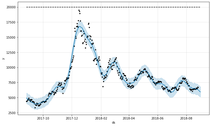
# 실제 데이터와 비교하기
# 예측데이터
pred_y = forecast_data.yhat.values[-5:]
pred_y

# array([6205.33466998, 6145.05228906, 6029.05388165, 5968.52723998,
#        5932.68137291])
# 실제데이터
test_file_path = 'market-price-test.csv'
bitcoin_test_df = pd.read_csv(test_file_path, names = ['ds', 'y'], header=0)
test_y = bitcoin_test_df.y.values
# 예측최소데이터
pred_y_lower = forecast_data.yhat_lower.values[-5:]

# 예측최대데이터
pred_y_upper = forecast_data.yhat_upper.values[-5:]
plt.plot(pred_y, color = 'gold') # 모델 예측한 가격그래프
plt.plot(pred_y_lower, color = 'red') # 모델이 예상한 최소 가격 그래프
plt.plot(pred_y_upper, color = 'blue') # 모델이 예상한 최대 가격 그래프
plt.plot(test_y, color = 'green') # 실제 가격 그래프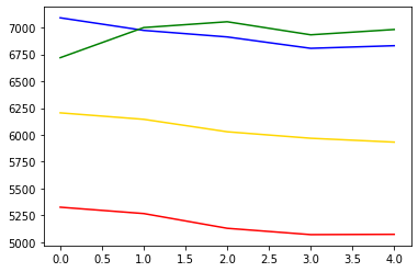
# 이상치 제거
bitcoin_df = pd.read_csv(file_path, names = ['ds', 'y'], header=0)
bitcoin_df.loc[bitcoin_df['y'] > 18000, 'y'] = None
bitcoin_df.info()
# 3건 제거

<class 'pandas.core.frame.DataFrame'>
RangeIndex: 365 entries, 0 to 364
Data columns (total 2 columns):
 #   Column  Non-Null Count  Dtype
---  ------  --------------  -----
 0   ds      365 non-null    object
 1   y       362 non-null    float64
dtypes: float64(1), object(1)
memory usage: 5.8+ KB
prophet = Prophet(seasonality_mode = 'multiplicative',
                 yearly_seasonality = True, # 연별
                 weekly_seasonality = True, # 주별
                 daily_seasonality = True, # 일별
                 changepoint_prior_scale = 0.5) # 과적합 방지 0.5만큼 만 분석
prophet.fit(bitcoin_df) # 학습하기
# 5일 앞을 예측하기
future_data = prophet.make_future_dataframe(periods=5, freq='d')
# # 상한가 설정
# future_data['cap'] = 20000
# 예측
forecast_data = prophet.predict(future_data)
forecast_data

	ds	trend	yhat_lower	yhat_upper	trend_lower	trend_upper	daily	daily_lower	daily_upper	multiplicative_terms	...	weekly	weekly_lower	weekly_upper	yearly	yearly_lower	yearly_upper	additive_terms	additive_terms_lower	additive_terms_upper	yhat
0	2017-08-27	528.085585	3766.698129	5075.496722	528.085585	528.085585	9.711762	9.711762	9.711762	7.371717	...	-0.109233	-0.109233	-0.109233	-2.230812	-2.230812	-2.230812	0.0	0.0	0.0	4420.983246
1	2017-08-28	529.776373	3961.128742	5121.531273	529.776373	529.776373	9.711762	9.711762	9.711762	7.479669	...	-0.054572	-0.054572	-0.054572	-2.177521	-2.177521	-2.177521	0.0	0.0	0.0	4492.328178
2	2017-08-29	531.467162	3978.374754	5172.827221	531.467162	531.467162	9.711762	9.711762	9.711762	7.642893	...	0.067545	0.067545	0.067545	-2.136414	-2.136414	-2.136414	0.0	0.0	0.0	4593.413651
3	2017-08-30	533.157950	4013.934349	5196.960495	533.157950	533.157950	9.711762	9.711762	9.711762	7.611159	...	0.009555	0.009555	0.009555	-2.110158	-2.110158	-2.110158	0.0	0.0	0.0	4591.108025
4	2017-08-31	534.848738	4008.172911	5178.939144	534.848738	534.848738	9.711762	9.711762	9.711762	7.647029	...	0.036189	0.036189	0.036189	-2.100922	-2.100922	-2.100922	0.0	0.0	0.0	4624.852670
...	...	...	...	...	...	...	...	...	...	...	...	...	...	...	...	...	...	...	...	...	...
365	2018-08-27	818.078684	6243.626452	7506.907764	818.078684	818.078684	9.711762	9.711762	9.711762	7.411506	...	-0.054572	-0.054572	-0.054572	-2.245684	-2.245684	-2.245684	0.0	0.0	0.0	6881.273946
366	2018-08-28	822.999668	6453.325229	7704.060396	822.999668	822.999668	9.711762	9.711762	9.711762	7.589491	...	0.067545	0.067545	0.067545	-2.189816	-2.189816	-2.189816	0.0	0.0	0.0	7069.148295
367	2018-08-29	827.920652	6419.908313	7727.754695	825.682414	827.920652	9.711762	9.711762	9.711762	7.575922	...	0.009555	0.009555	0.009555	-2.145395	-2.145395	-2.145395	0.0	0.0	0.0	7100.183131
368	2018-08-30	832.841636	6536.153516	7786.172133	823.752948	834.318783	9.711762	9.711762	9.711762	7.632749	...	0.036189	0.036189	0.036189	-2.115202	-2.115202	-2.115202	0.0	0.0	0.0	7189.713129
369	2018-08-31	837.762619	6550.207854	7952.370851	816.207036	850.803956	9.711762	9.711762	9.711762	7.688080	...	0.077855	0.077855	0.077855	-2.101537	-2.101537	-2.101537	0.0	0.0	0.0	7278.549033
370 rows × 22 columns
# 그래프로 작성
fig = prophet.plot(forecast_data)
# 실제 데이터와 비교하기
# 예측데이터
pred_y = forecast_data.yhat.values[-5:]
pred_y

# array([6881.2739463 , 7069.14829491, 7100.18313111, 7189.71312892,
#        7278.54903332])
# 실제데이터
test_file_path = 'market-price-test.csv'
bitcoin_test_df = pd.read_csv(test_file_path, names = ['ds', 'y'], header=0)
test_y = bitcoin_test_df.y.values

# 예측최소데이터
pred_y_lower = forecast_data.yhat_lower.values[-5:]

# 예측최대데이터
pred_y_upper = forecast_data.yhat_upper.values[-5:]
plt.plot(pred_y, color = 'gold') # 모델 예측한 가격그래프
plt.plot(pred_y_lower, color = 'red') # 모델이 예상한 최소 가격 그래프
plt.plot(pred_y_upper, color = 'blue') # 모델이 예상한 최대 가격 그래프
plt.plot(test_y, color = 'green') # 실제 가격 그래프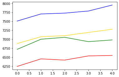
#
import numpy as np
import pandas as pd
import matplotlib.pyplot as plt
from fbprophet import Prophet
file_path = 'market-price.csv'
bitcoin_df = pd.read_csv(file_path, names = ['ds', 'y'], header=0)
# 상한가 설정
bitcoin_df['cap'] = 20000
# 하한가 설정
bitcoin_df['floor'] = 2000
# growth = logistic  상한설정시 추가, 비선형방식으로 분석
prophet = Prophet(seasonality_mode = 'multiplicative',
                  growth = 'logistic', # 상하한가 설정할때 , 비선형방식
                 yearly_seasonality = True, # 연별
                 weekly_seasonality = True, # 주별
                 daily_seasonality = True, # 일별
                 changepoint_prior_scale = 0.5) # 과적합 방지 0.5만큼 만 분석
prophet.fit(bitcoin_df) # 학습하기
# 5일 앞을 예측하기
future_data = prophet.make_future_dataframe(periods=5, freq='d')
# 상한가 설정
future_data['cap'] = 20000
future_data['floor'] = 2000
# 예측
forecast_data = prophet.predict(future_data)
forecast_data


ds	trend	cap	floor	yhat_lower	yhat_upper	trend_lower	trend_upper	daily	daily_lower	...	weekly	weekly_lower	weekly_upper	yearly	yearly_lower	yearly_upper	additive_terms	additive_terms_lower	additive_terms_upper	yhat
0	2017-08-27	5703.063125	20000	2000	3715.115421	5497.027367	5703.063125	5703.063125	0.426516	0.426516	...	0.003555	0.003555	0.003555	-0.626876	-0.626876	-0.626876	0.0	0.0	0.0	4580.676685
1	2017-08-28	5708.250950	20000	2000	3665.713289	5396.548303	5708.250950	5708.250950	0.426516	0.426516	...	-0.000994	-0.000994	-0.000994	-0.642812	-0.642812	-0.642812	0.0	0.0	0.0	4467.904518
2	2017-08-29	5713.444155	20000	2000	3501.918583	5273.509727	5713.444155	5713.444155	0.426516	0.426516	...	-0.000734	-0.000734	-0.000734	-0.659989	-0.659989	-0.659989	0.0	0.0	0.0	4375.317434
3	2017-08-30	5718.642741	20000	2000	3377.490794	5126.427715	5718.642741	5718.642741	0.426516	0.426516	...	-0.010622	-0.010622	-0.010622	-0.678244	-0.678244	-0.678244	0.0	0.0	0.0	4218.353837
4	2017-08-31	5723.846707	20000	2000	3284.264456	5033.597019	5723.846707	5723.846707	0.426516	0.426516	...	-0.008040	-0.008040	-0.008040	-0.697376	-0.697376	-0.697376	0.0	0.0	0.0	4127.470590
...	...	...	...	...	...	...	...	...	...	...	...	...	...	...	...	...	...	...	...	...	...
365	2018-08-27	7102.808324	20000	2000	4866.755803	6547.711110	7102.808324	7102.808324	0.426516	0.426516	...	-0.000994	-0.000994	-0.000994	-0.623101	-0.623101	-0.623101	0.0	0.0	0.0	5699.443947
366	2018-08-28	7106.076367	20000	2000	4743.519630	6436.151223	7106.076367	7106.076367	0.426516	0.426516	...	-0.000734	-0.000734	-0.000734	-0.638706	-0.638706	-0.638706	0.0	0.0	0.0	5593.025888
367	2018-08-29	7109.345673	20000	2000	4533.463676	6332.987745	7109.336045	7109.345673	0.426516	0.426516	...	-0.010622	-0.010622	-0.010622	-0.655587	-0.655587	-0.655587	0.0	0.0	0.0	5405.285348
368	2018-08-30	7112.616243	20000	2000	4408.976493	6155.807154	7112.547092	7112.630877	0.426516	0.426516	...	-0.008040	-0.008040	-0.008040	-0.673590	-0.673590	-0.673590	0.0	0.0	0.0	5298.091380
369	2018-08-31	7115.888076	20000	2000	4405.810985	6115.617608	7115.744311	7115.953331	0.426516	0.426516	...	0.000391	0.000391	0.000391	-0.692523	-0.692523	-0.692523	0.0	0.0	0.0	5225.796784
370 rows × 24 columns
# 그래프로 작성
fig = prophet.plot(forecast_data)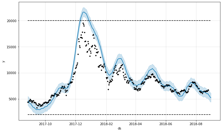
# 실제 데이터와 비교하기
# 예측데이터
pred_y = forecast_data.yhat.values[-5:]
pred_y

# array([5699.44394662, 5593.02588819, 5405.28534766, 5298.09137955,
#        5225.79678411])
# 실제데이터
test_file_path = 'market-price-test.csv'
bitcoin_test_df = pd.read_csv(test_file_path, names = ['ds', 'y'], header=0)
test_y = bitcoin_test_df.y.values

# 예측최소데이터
pred_y_lower = forecast_data.yhat_lower.values[-5:]

# 예측최대데이터
pred_y_upper = forecast_data.yhat_upper.values[-5:]
plt.plot(pred_y, color = 'gold') # 모델 예측한 가격그래프
plt.plot(pred_y_lower, color = 'red') # 모델이 예상한 최소 가격 그래프
plt.plot(pred_y_upper, color = 'blue') # 모델이 예상한 최대 가격 그래프
plt.plot(test_y, color = 'green') # 실제 가격 그래프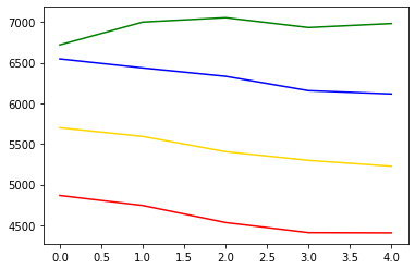
반응형
'Data_Science > Data_Analysis_Py' 카테고리의 다른 글
| 31. titanic || logistic (0) | 2021.11.24 |
|---|---|
| 30. 보스턴 주택가격정보 || 선형회귀 (0) | 2021.11.24 |
| 28. 비트코인 가격 시계열 분석 || Arima, fbProphet (0) | 2021.11.24 |
| 27. 프로야구 연봉 예측 분석 || OLS, Heatmap (0) | 2021.11.24 |
| 26. 서울 중학교 졸업자 분석 || dbscan, folium (0) | 2021.11.24 |