728x90
반응형
OpenCV
Hisogram
이미지 데이터를 분석하기 위한 방법으로 사용한다
import cv2
import numpy as np

im = cv2.imread('people.jpg')
cv2.calcHist([im],[0], None, [256], [0,256]) # 여러개 동시에 연산하기 때문에 2차로 결과를 낸다
cv2.calcHist([im,im],[0], None, [256], [0,256])

# 색상 분포
plt.plot(cv2.calcHist([im],[0], None, [256], [0,256])) # B
plt.plot(cv2.calcHist([im],[1], None, [256], [0,256])) # G
plt.plot(cv2.calcHist([im],[2], None, [256], [0,256])) # R
plt.xlim([0, 256])
# (0.0, 256.0)
squeeze
길이가 1 인 축을 제거한다
a = np.array([[1],[3]])
b = np.array([[[1,2],[3,4]]])

a.shape, b.shape
# ((2, 1), (1, 2, 2))

np.squeeze(a).shape, np.squeeze(b).shape
# ((2,), (2, 2))

cv2.calcHist([im,im],[0], None, [256], [0,256]).shape
# (256, 1)

np.squeeze(cv2.calcHist([im,im],[0], None, [256], [0,256])).shape
# (256,)

plt.plot(cv2.calcHist([im,im],[0], None, [256], [0,256]))
plt.plot(cv2.calcHist([im,im],[1], None, [256], [0,256]))
plt.plot(cv2.calcHist([im,im],[2], None, [256], [0,256]))
속도 비교
opencv는 속도 최적화가 되어 있다
%timeit im*im
# 1000 loops, best of 5: 202 µs per loop

%timeit im**2
# 1000 loops, best of 5: 227 µs per loop

cv2.useOptimized() # opencv연산에 최적화 되어 있다
# True

%timeit cv2.medianBlur(im, 49) # 최적화 되어 있을 때 (최적화 되어 있을 때 일반적으로 20% 빠르다 / colab에서 medianBlur연산은 최적화 해도 그렇게 빠르지 않다)
# 10 loops, best of 5: 37.5 ms per loop

cv2.setUseOptimized(False)
cv2.useOptimized()
# False

%timeit cv2.medianBlur(im, 49) # 최적화 되지 않을 때
# 10 loops, best of 5: 37.8 ms per loop

cv2.setUseOptimized(True)
cv2.useOptimized()
# True

%timeit im*im*im
# The slowest run took 20.40 times longer than the fastest. This could mean that an intermediate result is being cached.
# 1000 loops, best of 5: 292 µs per loop

%timeit im**3 # 연산량이 많아지면서 im*im*im연산보다 im**3이 훨씬 느려졌다
# 100 loops, best of 5: 3.24 ms per loop
EqualizeHist
im = cv2.imread('people.jpg', 0)
im2 = cv2.equalizeHist(im)

plt.hist(im2.ravel(), 256,[0,256]); # 정규 분포 처럼 분포를 균일하게 만들어 준다
plt.imshow(cv2.equalizeHist(im), cmap='gray') # 평탄화 => contrast가 낮아진다 => 분포가 균일해진다 => 밝고 어두운 정도가 구분하기 힘들어진다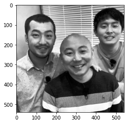
from skimage.exposure import cumulative_distribution
len(cumulative_distribution(im))
# 2

y, x = cumulative_distribution(im)
plt.hist(y);
# (array([ 26.,  29.,  48.,  28.,  17.,  13.,  12.,  13.,  16.,  54.]),
#  array([  2.74348422e-05,   1.00024691e-01,   2.00021948e-01,
#           3.00019204e-01,   4.00016461e-01,   5.00013717e-01,
#           6.00010974e-01,   7.00008230e-01,   8.00005487e-01,
#           9.00002743e-01,   1.00000000e+00]),
#  <a list of 10 Patch objects>)
plt.plot(x,y) # 누적 분포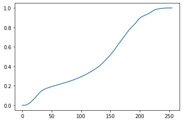
Numpy
Histogram
import matplotlib.pyplot as plt
im = cv2.imread('people.jpg') # color
np.histogram(im, bins=10) # return이 두 개 (hist array, bin_edges(length(hist)+1)
# (array([ 78609,  83722,  55425,  62639,  96251, 126726, 146684, 112897, 90637,  21210]),
# array([   0. ,   25.5,   51. ,   76.5,  102. ,  127.5,  153. ,  178.5, 204. ,  229.5,  255. ]))

im.dtype # 2^8 = 256
# dtype('uint8')
np.histogram(im, bins=256, range=[0,256]) # 256등분 / 0이 92개 1이 51개... / color정보이기 때문에 수치가 많이 나온다
(array([ 92, 51, 119, 224, 406, 664, 1290, 1818, 2323, 2826, 3018,
3290, 3549, 3736, 3856, 3928, 4209, 4413, 4537, 4848, 4852, 4987,
5005, 4958, 4881, 4729, 4570, 4256, 4186, 3976, 3849, 3605, 3503,
3489, 3487, 3281, 3249, 3110, 3217, 3150, 3008, 3073, 3052, 3206,
3193, 3086, 3089, 2943, 2895, 2695, 2554, 2507, 2258, 2389, 2191,
2185, 2115, 2019, 2163, 2048, 2012, 1996, 2055, 2095, 2010, 2032,
2135, 2132, 2138, 2077, 2140, 2097, 2144, 2098, 2128, 2106, 2155,
2202, 2166, 2168, 2230, 2255, 2285, 2306, 2289, 2345, 2337, 2360,
2358, 2429, 2430, 2487, 2562, 2697, 2688, 2753, 2745, 2776, 2783,
2924, 2969, 3095, 3149, 3179, 3199, 3258, 3302, 3349, 3284, 3369,
3413, 3501, 3640, 3540, 3542, 3759, 3692, 3722, 3801, 3801, 3971,
3999, 4021, 4278, 4239, 4254, 4480, 4509, 4408, 4414, 4677, 4674,
4743, 4873, 5055, 5089, 5088, 5225, 5319, 5080, 5087, 5054, 5099,
5108, 4934, 5152, 5206, 5158, 5211, 5364, 5454, 5661, 5593, 5789,
5680, 5836, 6015, 6139, 6026, 6087, 6087, 6021, 5803, 5809, 5856,
5577, 5669, 5457, 5222, 5190, 5102, 5128, 5095, 5237, 5525, 5453,
5417, 5741, 5723, 5894, 5497, 5167, 5182, 4995, 5002, 4729, 4781,
4483, 4499, 4386, 4289, 4507, 4544, 4808, 4740, 4456, 4135, 4062,
4144, 3972, 3651, 3572, 3636, 3766, 3982, 4385, 4202, 3822, 3792,
3704, 3515, 3518, 3573, 3704, 3808, 4347, 3945, 3734, 3859, 3718,
3615, 3450, 3275, 2991, 3032, 2811, 2796, 2627, 2314, 2118, 2154,
1870, 1627, 1593, 1576, 1468, 1315, 1319, 1145, 1057, 959, 866,
745, 614, 560, 469, 383, 319, 242, 217, 175, 144, 105,
70, 53, 165]),
array([ 0., 1., 2., 3., 4., 5., 6., 7., 8.,
9., 10., 11., 12., 13., 14., 15., 16., 17.,
18., 19., 20., 21., 22., 23., 24., 25., 26.,
27., 28., 29., 30., 31., 32., 33., 34., 35.,
36., 37., 38., 39., 40., 41., 42., 43., 44.,
45., 46., 47., 48., 49., 50., 51., 52., 53.,
54., 55., 56., 57., 58., 59., 60., 61., 62.,
63., 64., 65., 66., 67., 68., 69., 70., 71.,
72., 73., 74., 75., 76., 77., 78., 79., 80.,
81., 82., 83., 84., 85., 86., 87., 88., 89.,
90., 91., 92., 93., 94., 95., 96., 97., 98.,
99., 100., 101., 102., 103., 104., 105., 106., 107.,
108., 109., 110., 111., 112., 113., 114., 115., 116.,
117., 118., 119., 120., 121., 122., 123., 124., 125.,
126., 127., 128., 129., 130., 131., 132., 133., 134.,
135., 136., 137., 138., 139., 140., 141., 142., 143.,
144., 145., 146., 147., 148., 149., 150., 151., 152.,
153., 154., 155., 156., 157., 158., 159., 160., 161.,
162., 163., 164., 165., 166., 167., 168., 169., 170.,
171., 172., 173., 174., 175., 176., 177., 178., 179.,
180., 181., 182., 183., 184., 185., 186., 187., 188.,
189., 190., 191., 192., 193., 194., 195., 196., 197.,
198., 199., 200., 201., 202., 203., 204., 205., 206.,
207., 208., 209., 210., 211., 212., 213., 214., 215.,
216., 217., 218., 219., 220., 221., 222., 223., 224.,
225., 226., 227., 228., 229., 230., 231., 232., 233.,
234., 235., 236., 237., 238., 239., 240., 241., 242.,
243., 244., 245., 246., 247., 248., 249., 250., 251.,
252., 253., 254., 255., 256.]))np.histogram(im.flatten(), 256, [0,256]) # flatten함수는 일차원으로 바꿔주는 함수 => 연산을 더 빠르게 하기 위해서 바꾼다
(array([ 92, 51, 119, 224, 406, 664, 1290, 1818, 2323, 2826, 3018,
3290, 3549, 3736, 3856, 3928, 4209, 4413, 4537, 4848, 4852, 4987,
5005, 4958, 4881, 4729, 4570, 4256, 4186, 3976, 3849, 3605, 3503,
3489, 3487, 3281, 3249, 3110, 3217, 3150, 3008, 3073, 3052, 3206,
3193, 3086, 3089, 2943, 2895, 2695, 2554, 2507, 2258, 2389, 2191,
2185, 2115, 2019, 2163, 2048, 2012, 1996, 2055, 2095, 2010, 2032,
2135, 2132, 2138, 2077, 2140, 2097, 2144, 2098, 2128, 2106, 2155,
2202, 2166, 2168, 2230, 2255, 2285, 2306, 2289, 2345, 2337, 2360,
2358, 2429, 2430, 2487, 2562, 2697, 2688, 2753, 2745, 2776, 2783,
2924, 2969, 3095, 3149, 3179, 3199, 3258, 3302, 3349, 3284, 3369,
3413, 3501, 3640, 3540, 3542, 3759, 3692, 3722, 3801, 3801, 3971,
3999, 4021, 4278, 4239, 4254, 4480, 4509, 4408, 4414, 4677, 4674,
4743, 4873, 5055, 5089, 5088, 5225, 5319, 5080, 5087, 5054, 5099,
5108, 4934, 5152, 5206, 5158, 5211, 5364, 5454, 5661, 5593, 5789,
5680, 5836, 6015, 6139, 6026, 6087, 6087, 6021, 5803, 5809, 5856,
5577, 5669, 5457, 5222, 5190, 5102, 5128, 5095, 5237, 5525, 5453,
5417, 5741, 5723, 5894, 5497, 5167, 5182, 4995, 5002, 4729, 4781,
4483, 4499, 4386, 4289, 4507, 4544, 4808, 4740, 4456, 4135, 4062,
4144, 3972, 3651, 3572, 3636, 3766, 3982, 4385, 4202, 3822, 3792,
3704, 3515, 3518, 3573, 3704, 3808, 4347, 3945, 3734, 3859, 3718,
3615, 3450, 3275, 2991, 3032, 2811, 2796, 2627, 2314, 2118, 2154,
1870, 1627, 1593, 1576, 1468, 1315, 1319, 1145, 1057, 959, 866,
745, 614, 560, 469, 383, 319, 242, 217, 175, 144, 105,
70, 53, 165]),
array([ 0., 1., 2., 3., 4., 5., 6., 7., 8.,
9., 10., 11., 12., 13., 14., 15., 16., 17.,
18., 19., 20., 21., 22., 23., 24., 25., 26.,
27., 28., 29., 30., 31., 32., 33., 34., 35.,
36., 37., 38., 39., 40., 41., 42., 43., 44.,
45., 46., 47., 48., 49., 50., 51., 52., 53.,
54., 55., 56., 57., 58., 59., 60., 61., 62.,
63., 64., 65., 66., 67., 68., 69., 70., 71.,
72., 73., 74., 75., 76., 77., 78., 79., 80.,
81., 82., 83., 84., 85., 86., 87., 88., 89.,
90., 91., 92., 93., 94., 95., 96., 97., 98.,
99., 100., 101., 102., 103., 104., 105., 106., 107.,
108., 109., 110., 111., 112., 113., 114., 115., 116.,
117., 118., 119., 120., 121., 122., 123., 124., 125.,
126., 127., 128., 129., 130., 131., 132., 133., 134.,
135., 136., 137., 138., 139., 140., 141., 142., 143.,
144., 145., 146., 147., 148., 149., 150., 151., 152.,
153., 154., 155., 156., 157., 158., 159., 160., 161.,
162., 163., 164., 165., 166., 167., 168., 169., 170.,
171., 172., 173., 174., 175., 176., 177., 178., 179.,
180., 181., 182., 183., 184., 185., 186., 187., 188.,
189., 190., 191., 192., 193., 194., 195., 196., 197.,
198., 199., 200., 201., 202., 203., 204., 205., 206.,
207., 208., 209., 210., 211., 212., 213., 214., 215.,
216., 217., 218., 219., 220., 221., 222., 223., 224.,
225., 226., 227., 228., 229., 230., 231., 232., 233.,
234., 235., 236., 237., 238., 239., 240., 241., 242.,
243., 244., 245., 246., 247., 248., 249., 250., 251.,
252., 253., 254., 255., 256.]))일차원으로 만드는 함수
1. ravel # view 방식
2. flatten # copy 방식
plt.hist(im.ravel(), 256, [0, 256]); # 내부적으로 bincount를 사용해서 연산한다
plt.xlim([0,256]) # x축 범위 설정
im2 = cv2.imread('people.jpg', 0) # 흑백
plt.hist(im2.flatten(), 256, [0, 256]);
plt.xlim([0,256])
# (0.0, 256.0)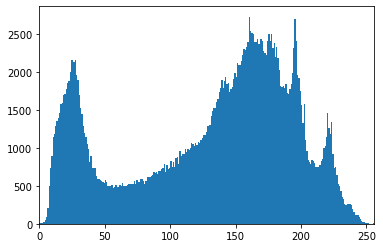
# 각각 점의 컬러 분포
plt.hist(im[...,0].ravel(), 256, [0, 256]); # B
plt.hist(im[...,1].ravel(), 256, [0, 256]); # G
plt.hist(im[...,2].ravel(), 256, [0, 256]); # R
plt.xlim([0,256])
im2.shape # 흑백
# (540, 540)
im2
# array([[191, 193, 194, ..., 165, 166, 168],
#       [190, 192, 193, ..., 173, 175, 176],
#       [189, 191, 192, ..., 182, 183, 184],
#       ...,
#       [106, 102, 109, ..., 113, 124, 129],
#       [106, 102, 109, ..., 113, 120, 123],
#       [101,  97, 104, ..., 119, 120, 120]], dtype=uint8)

plt.hist(im2[0].flatten(), 256, [0, 256]);
plt.hist(im2[1].flatten(), 256, [0, 256]);
plt.hist(im2[539].flatten(), 256, [0, 256]);
plt.xlim([0,256])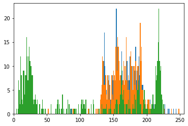
np.bincount(np.arange(5)) # 각각 몇개 있는지 세는 함수
# array([1, 1, 1, 1, 1])

np.bincount(np.array([0,1,1,3,2,1,7]))
# array([1, 3, 1, 1, 0, 0, 0, 1])

from itertools import count, groupby
t = groupby([1,1,1,2,2])
b = count()
next(b)
# 3

next(t) # 그룹으로 묶어서 몇개 있는지 확인
# (2, <itertools._grouper at 0x7fa251080ad0>)
얼굴부분 crop해서 색 분포 확인하기
face = im[50:300,50:200]
plt.imshow(face[...,::-1])
plt.hist(face[...,0].ravel(), 256, [0, 256], color='blue');
plt.hist(face[...,1].ravel(), 256, [0, 256], color='green');
plt.hist(face[...,2].ravel(), 256, [0, 256], color='red');
plt.xlim([0,256])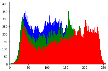
mask = np.zeros(im.shape[:2], np.uint8) # mask
mask[50:300,50:200] = 255 # 흰색으로
cv2.bitwise_and(im,im,mask=mask)
plt.imshow(cv2.bitwise_and(im,im,mask=mask))
plt.imshow(cv2.bitwise_and(im,mask)) # 차원이 달라서 연산이 안된다
# error: OpenCV(4.1.2) /io/opencv/modules/core/src/arithm.cpp:229: error: (-209:Sizes of input arguments do not match) The operation is neither 'array op array' (where arrays have the same size and type), nor 'array op scalar', nor 'scalar op array' in function 'binary_op'
im.shape, mask.shape
# ((540, 540, 3), (540, 540))
im2 = cv2.imread('people.jpg', 0)
plt.imshow(cv2.bitwise_and(im2,mask))
cv2.calcHist([im], [0], mask, [256], [0,256]) # mask외 분포 구할 때
plt.plot(cv2.calcHist([im], [0], mask, [256], [0,256]))
전통적인 머신러닝에서는 contrast가 높으면 이미지 분류가 잘 안되기 때문에 contrast 분포를 평평하게 만들었었다 (contrast normalization)
from skimage.exposure import histogram, rescale_intensity, equalize_hist
from skimage.util import img_as_float, img_as_ubyte
im = cv2.imread('people.jpg')
plt.imshow(img_as_float(im)[...,::-1])
# 이미지는 float나 int 둘다 사람이 볼때는 상관 없다 / 하지만 컴퓨터는 float로 바꾸면 연속적이기 때문에 미분이 가능해진다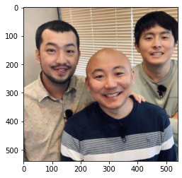
help(histogram)
np.info(histogram)
np.lookfor('hist', 'skimage')
import scipy
np.lookfor('hist', 'scipy')equalize_hist(im.flatten())
# array([ 0.73654893, 0.80552241, 0.86368427, ..., 0.47972908, 0.42027549, 0.32775834])plt.imshow(rescale_intensity(im, (0, 255))) # 범위를 조절 해준다
plt.imshow(rescale_intensity(im[...,::-1], (0, 255)))
plt.imshow(rescale_intensity(im[...,::-1], (0, 50))) # 0에서 50사이로 범위를 조절 했기 때문에 밝게 변한다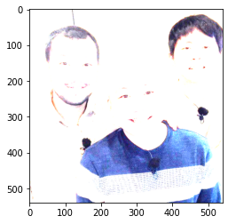
plt.imshow(rescale_intensity(im[...,::-1], (, 200)))advanced
x = [1,2,3,4,5,6]
y = np.array(x)

y.cumsum() # 누적합을 빠르게 구하는 방법
# array([ 1,  3,  6, 10, 15, 21])

np.add.accumulate(y)
# array([ 1,  3,  6, 10, 15, 21])

np.add.reduce(y)
# 21
import tensorflow as tf
tf.reduce_sum(y)
# <tf.Tensor: shape=(), dtype=int64, numpy=21>
# import seaborn as sns
iris = sns.load_dataset('iris')
sns.pairplot(iris, hue='species', diag_kind='hist') # 데이터에 분포에 따라서 옳바른 데이터인지 아닌지 확인할 수 있기 때문에 그래프를 확인한다
sns.pairplot(iris, hue='species', diag_kind='kde')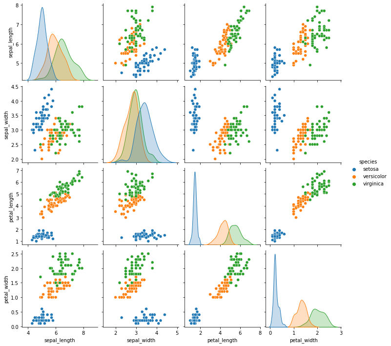
누적 분포
hist, bins = np.histogram(im.ravel(), 256, [0,256])
cdf = hist.cumsum()

cdf_norm = cdf*float(hist.max()) / cdf.max() # 정규화, 0과 1사이의 값으로 만든다

plt.hist(im.ravel(), 256, [0,256])
plt.plot(cdf_norm)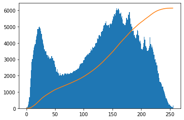
반응형
'Computer_Science > Visual Intelligence' 카테고리의 다른 글
| 11일차 - 영상 데이터 기계학습 활용 (0) | 2021.09.26 |
|---|---|
| 9일차 - 영상 데이터 기계학습 활용 (0) | 2021.09.21 |
| 8일차 - Image 처리 (3) (1) | 2021.09.21 |
| 7일차 - Image 처리 (2) (0) | 2021.09.21 |
| 6일차 - Image 처리 (1) (0) | 2021.09.21 |