Computer Vision Footprint
1998 - LeNet 5
2012 - AlexNet
- Gradient vanishin문제를 해결하는 ReLU를 사용 - LRN 사용 안했음
- Overlapping Pooling(영향력이 크진 않음)
- Dropout(Overfitting 방지)
2013 - ZFNet
- AlexNet을 Visualization통해 insight를 제공
- HyperParameter tuning 방법론 제시
- Network in Network
- 1x1 Convolution 도입 (1. 차원 조절 2. non-linear 특성 부여 3. fully connected 처럼 사용)
- Flatten 대신 사용하는 방법인 Global Average Pooling 도입
- 같은 형태를 반복하고 겹쳐서 사용하는 Stacking 도입
2014 - GoogLeNet v1 (1등)
- 1x1 convolution 활용
- Inception module stacking
- Global average pooling 활용
- VGG (2등)
2016 - GoogLeNet v4
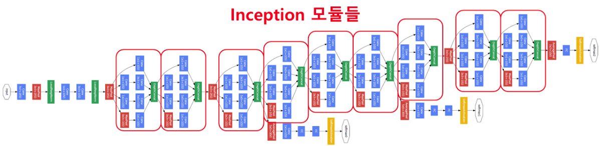
GoogLeNet
ReLU와 같은 기법 덕에 Layer를 깊게 쌓을 수 있는 확신이 있었던 배경 때문에 Layer를 어떻게 깊게 쌓는지 여부가 중요한 포인트였다
GoogLeNet 특징
1. 1x1 convolution
- 차원 축소 효과
- nonlinearity 특징 부여
2. Inception module
- 9개 inception module로 구성되어 있다
- Inception moddule은 Hebbian rule에 의해 영향력이 가장 큰 부분이 연결성이 강화된다(weight가 커진다)
- 실제 구현에서는 차원을 조절하여 inception module을 적용하였다
3. Global average pooling
4. Auxiliary classifier
- relu로 gradient vanishing 문제를 해결한듯 했으나 layer가 기존에 8 layer였던것에 비해 22 layer로 급격하게 늘었기 때문에 gradient vanishing 가능성이 생겼다
- 따라서 네트워크 중간에 auxiliary classifier를 추가하여 중간 중간 결과를 낸다
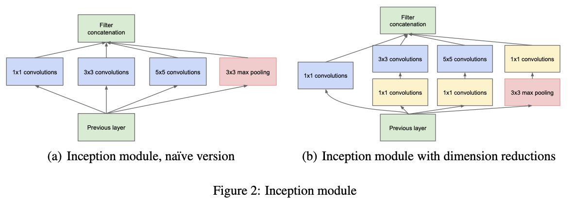
Inception module
import tensorflow as tf

(X_train, y_train), (X_test, y_test) = tf.keras.datasets.cifar10.load_data()

# Inception module, naive version
input_ = tf.keras.Input((32,32,3))
conv1x1 = tf.keras.layers.Conv2D(3,1, padding='same', name='1x1')(input_)
conv3x3 = tf.keras.layers.Conv2D(3,3, padding='same', name='3x3')(input_)
conv5x5 = tf.keras.layers.Conv2D(3,3, padding='same', name='5x5')(input_)
maxpool = tf.keras.layers.MaxPool2D(3,1, padding='same', name='pool')(input_) # unoverlapping
concatenate = tf.keras.layers.Concatenate()([conv1x1,conv3x3,conv5x5,maxpool]) # 합치기 위해서 구조를 맞추어야 한다

model = tf.keras.models.Model(input_, concatenate)
model.summary()
# Model: "model_13"
# __________________________________________________________________________________________________
# Layer (type) Output Shape Param # Connected to
# ==================================================================================================
# input_24 (InputLayer) [(None, 32, 32, 3)] 0
# __________________________________________________________________________________________________
# 1x1 (Conv2D) (None, 32, 32, 3) 12 input_24[0][0]
# __________________________________________________________________________________________________
# 3x3 (Conv2D) (None, 32, 32, 3) 84 input_24[0][0]
# __________________________________________________________________________________________________
# 5x5 (Conv2D) (None, 32, 32, 3) 84 input_24[0][0]
# __________________________________________________________________________________________________
# pool (MaxPooling2D) (None, 32, 32, 3) 0 input_24[0][0]
# __________________________________________________________________________________________________
# concatenate_15 (Concatenate) (None, 32, 32, 12) 0 1x1[0][0]
# 3x3[0][0]
# 5x5[0][0]
# pool[0][0]
# ==================================================================================================
# Total params: 180
# Trainable params: 180
# Non-trainable params: 0
# __________________________________________________________________________________________________tf.keras.utils.plot_model(model, show_shapes=True)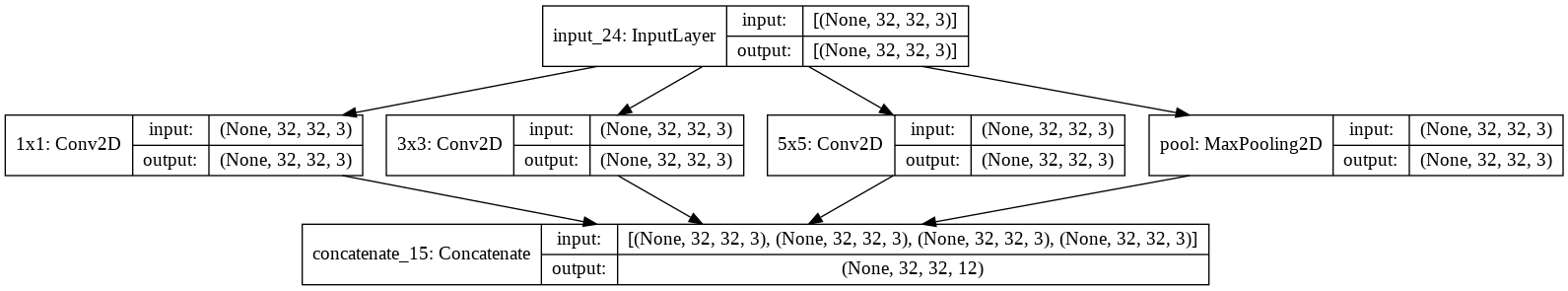
# Inception module with dimension reductions
input_ = tf.keras.Input((32,32,3))
conv1x1 = tf.keras.layers.Conv2D(3,1, padding='same', name='1x1')(input_)
conv1x1_reduc3x3 = tf.keras.layers.Conv2D(2,1, padding='same', name='1x1_3x3')(input_)
conv3x3 = tf.keras.layers.Conv2D(2,3, padding='same', name='3x3')(conv1x1_reduc3x3)
conv1x1_reduc5x5 = tf.keras.layers.Conv2D(2,1, padding='same', name='1x1_5x5')(input_)
conv5x5 = tf.keras.layers.Conv2D(2,3, padding='same', name='5x5')(conv1x1_reduc5x5)
maxpool = tf.keras.layers.MaxPool2D(2,1, padding='same', name='pool')(input_)
conv1x1_reduc_mp = tf.keras.layers.Conv2D(2,1, padding='same', name='1x1_pool')(maxpool)
concatenate = tf.keras.layers.Concatenate(axis=-1)([conv1x1,conv3x3,conv5x5,conv1x1_reduc_mp]) # 합치기 위해서 구조를 맞추어야 한다
# concatenate = tf.keras.layers.Concatenate([conv1x1,conv3x3,conv5x5,conv1x1_reduc_mp]) # 옵션을 주지 않을때

model = tf.keras.models.Model(input_, concatenate)
model.summary()
# Model: "model_14"
# __________________________________________________________________________________________________
# Layer (type) Output Shape Param # Connected to
# ==================================================================================================
# input_25 (InputLayer) [(None, 32, 32, 3)] 0
# __________________________________________________________________________________________________
# 1x1_3x3 (Conv2D) (None, 32, 32, 2) 8 input_25[0][0]
# __________________________________________________________________________________________________
# 1x1_5x5 (Conv2D) (None, 32, 32, 2) 8 input_25[0][0]
# __________________________________________________________________________________________________
# pool (MaxPooling2D) (None, 32, 32, 3) 0 input_25[0][0]
# __________________________________________________________________________________________________
# 1x1 (Conv2D) (None, 32, 32, 3) 12 input_25[0][0]
# __________________________________________________________________________________________________
# 3x3 (Conv2D) (None, 32, 32, 2) 38 1x1_3x3[0][0]
# __________________________________________________________________________________________________
# 5x5 (Conv2D) (None, 32, 32, 2) 38 1x1_5x5[0][0]
# __________________________________________________________________________________________________
# 1x1_pool (Conv2D) (None, 32, 32, 2) 8 pool[0][0]
# __________________________________________________________________________________________________
# concatenate_16 (Concatenate) (None, 32, 32, 9) 0 1x1[0][0]
# 3x3[0][0]
# 5x5[0][0]
# 1x1_pool[0][0]
# ==================================================================================================
# Total params: 112
# Trainable params: 112
# Non-trainable params: 0
# __________________________________________________________________________________________________tf.keras.utils.plot_model(model, show_shapes=True, rankdir="BT", show_dtype=True) # wide하게 분포되어 있기 때문에 parameter operator가 엄청 많다 / 이중에서 영향력 있는 것만 강한 연결성을 띄게 된다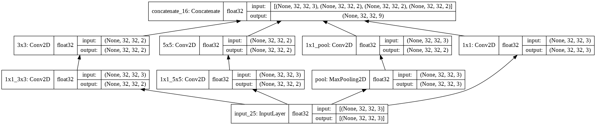
in3 = tf.keras.applications.InceptionV3()

tf.keras.utils.plot_model(in3)
Visual Geometry Group
Very Deep Convolutional Networks for large-scale image recognition
Layer가 깊어지면 깊어질 수 록 성능이 좋아진다
Abliation study 방식으로 모델 성능을 비교한다
1. AlexNet vs AlexNet + LRN
- LRN 기법은 성능 개선은 없고 메모리 사용량 및 연산 시간만 늘어났기에 사용을 하지 않는다
2. AlexNet vs AlexNet + conv layer 2개 추가
- 성능 좋아짐
3. AlexNet + conv layer 2개 vs AlexNet + conv layer 2개 + 1x1 convolution 3개
- Nonlinearity만 추가 시켜 성능향상을 하는지 확인 => activation이 더 많아서 성능 더 좋아짐 (UAT)
4. AlexNet + conv layer 2개 + 1x1 convolution 3개 vs AlexNet + conv layer 5개
- 성능 좋아짐
5. AlexNet + conv layer 5개 vs AlexNet + conv layer 8개
- 성능 좋아짐
결국 Layer가 늘어나면 늘어날 수록 성능이 좋아졌다
model을 불러와 사용하는 두 가지 방식
1. applications => Computer vision 분야에서 지원되는 모델을 지원한다
2. tensorflow hub
import tensorflow as tf

vgg16 = tf.keras.applications.VGG16() # ImageNet 대회서 2등, 학습된 모델을 그대로 사용할 수 있다

vgg16.summary()
# Model: "vgg16"
# _________________________________________________________________
# Layer (type)                 Output Shape              Param #
# =================================================================
# input_2 (InputLayer)         [(None, 224, 224, 3)]     0
# _________________________________________________________________
# block1_conv1 (Conv2D)        (None, 224, 224, 64)      1792
# _________________________________________________________________
# block1_conv2 (Conv2D)        (None, 224, 224, 64)      36928
# _________________________________________________________________
# block1_pool (MaxPooling2D)   (None, 112, 112, 64)      0
# _________________________________________________________________
# block2_conv1 (Conv2D)        (None, 112, 112, 128)     73856
# _________________________________________________________________
# block2_conv2 (Conv2D)        (None, 112, 112, 128)     147584
# _________________________________________________________________
# block2_pool (MaxPooling2D)   (None, 56, 56, 128)       0
# _________________________________________________________________
# block3_conv1 (Conv2D)        (None, 56, 56, 256)       295168
# _________________________________________________________________
# block3_conv2 (Conv2D)        (None, 56, 56, 256)       590080
# _________________________________________________________________
# block3_conv3 (Conv2D)        (None, 56, 56, 256)       590080
# _________________________________________________________________
# block3_pool (MaxPooling2D)   (None, 28, 28, 256)       0
# _________________________________________________________________
# block4_conv1 (Conv2D)        (None, 28, 28, 512)       1180160
# _________________________________________________________________
# block4_conv2 (Conv2D)        (None, 28, 28, 512)       2359808
# _________________________________________________________________
# block4_conv3 (Conv2D)        (None, 28, 28, 512)       2359808
# _________________________________________________________________
# block4_pool (MaxPooling2D)   (None, 14, 14, 512)       0
# _________________________________________________________________
# block5_conv1 (Conv2D)        (None, 14, 14, 512)       2359808
# _________________________________________________________________
# block5_conv2 (Conv2D)        (None, 14, 14, 512)       2359808
# _________________________________________________________________
# block5_conv3 (Conv2D)        (None, 14, 14, 512)       2359808
# _________________________________________________________________
# block5_pool (MaxPooling2D)   (None, 7, 7, 512)         0
# _________________________________________________________________
# flatten (Flatten)            (None, 25088)             0
# _________________________________________________________________
# fc1 (Dense)                  (None, 4096)              102764544
# _________________________________________________________________
# fc2 (Dense)                  (None, 4096)              16781312
# _________________________________________________________________
# predictions (Dense)          (None, 1000)              4097000
# =================================================================
# Total params: 138,357,544
# Trainable params: 138,357,544
# Non-trainable params: 0
# _________________________________________________________________
vgg16.weights
vgg16.__class__
# keras.engine.functional.Functional3x3을 쓰는 이유
(X_train, y_train), (X_test, y_test) = tf.keras.datasets.cifar10.load_data()

input_ = tf.keras.Input((32,32,3))
x = tf.keras.layers.Conv2D(2,5)(input_) # filter 2개 5x5
model = tf.keras.models.Model(input_, x)

model.summary()
# Model: "model"
# _________________________________________________________________
# Layer (type)                 Output Shape              Param #
# =================================================================
# input_4 (InputLayer)         [(None, 32, 32, 3)]       0
# _________________________________________________________________
# conv2d (Conv2D)              (None, 28, 28, 2)         152
# =================================================================
# Total params: 152
# Trainable params: 152
# Non-trainable params: 0
# _________________________________________________________________
input_ = tf.keras.Input((32,32,3))
x = tf.keras.layers.Conv2D(2,3)(input_)
x = tf.keras.layers.Conv2D(2,3)(x)
model = tf.keras.models.Model(input_, x)
model.summary() # 3x3이 더 좋다 / 5x5일 때와 shape은 같지만 activation을 여러개 사용했고 파라미터 수가 줄어들었기 때문에 성능이 더 좋아졌다
# Model: "model_15"
# _________________________________________________________________
# Layer (type) Output Shape Param #
# =================================================================
# input_27 (InputLayer) [(None, 32, 32, 3)] 0
# _________________________________________________________________
# conv2d_221 (Conv2D) (None, 30, 30, 2) 56
# _________________________________________________________________
# conv2d_222 (Conv2D) (None, 28, 28, 2) 38
# =================================================================
# Total params: 94
# Trainable params: 94
# Non-trainable params: 0
# _________________________________________________________________input_ = tf.keras.Input((32,32,3))
x = tf.keras.layers.Conv2D(2,3)(input_)
x = tf.keras.layers.Conv2D(2,3)(x)
x = tf.keras.layers.Conv2D(2,3)(x)
model = tf.keras.models.Model(input_, x)
model.summary() # 3x3으로 더 큰 receptive field를 대체 할 수 있다
# Model: "model_24"
# _________________________________________________________________
# Layer (type) Output Shape Param #
# =================================================================
# input_36 (InputLayer) [(None, 32, 32, 3)] 0
# _________________________________________________________________
# conv2d_243 (Conv2D) (None, 30, 30, 2) 56
# _________________________________________________________________
# conv2d_244 (Conv2D) (None, 28, 28, 2) 38
# _________________________________________________________________
# conv2d_245 (Conv2D) (None, 26, 26, 2) 38
# =================================================================
# Total params: 132
# Trainable params: 132
# Non-trainable params: 0
# _________________________________________________________________보통 첫번째 layer는 5x5 또는 7x7 filter를 사용하고
(처음부터 3x3을 사용하면 메모리를 너무 많이차지 하기 때문에 오히려 성능 저하가 될 수 있다)
그 다음 layer 부터는 3x3을 사용하면 성능이 좋다
Deep Residual Learning for Image Recognition
ResNet은 인간을 뛰어넘은 첫번째 모델
Residual => 실제값 - 예측값 (잔차)
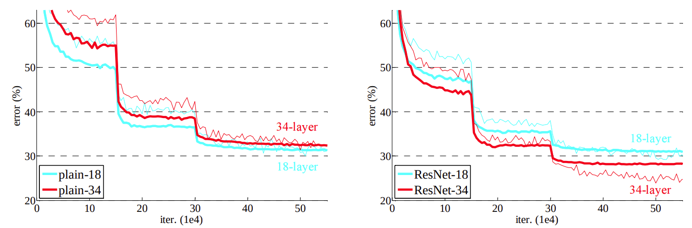
layer가 56개로 깊어지면서 gradient vanishing문제가 다시 떠오르기 시작했다
(relu로 해결되지 못하는 문제가 발생) underfitting
처음에 학습했던 것들을 점차 잊게되면서 목표로 부터 멀어지게 되는 현상이 생겼다
그래서 해결책으로 Short cut 즉, residual block을 도입하게 되었다
LSTM에서 아이디어를 얻어 자신의 값을 더함으로써 값을 유지시키고 목표를 잃지 않고 지속적으로 학습하게 된다
기존의 신경망은 입력값 x를 타겟값 y로 매핑하는 함수 H(x)를 얻는 것이 목적이었다.
그러나 ResNet은 F(x) + x를 최소화하는 것을 목적으로 한다.
x는 현시점에서 변할 수 없는 값이므로 F(x)를 0에 가깝게 만드는 것이 목적이 된다.
F(x)가 0이 되면 출력과 입력이 모두 x로 같아지게 된다.
F(x) = H(x) - x이므로 F(x)를 최소로 해준다는 것은 H(x) - x를 최소로 해주는 것과 동일한 의미를 지닌다.
여기서 H(x) - x를 잔차(residual)라고 한다.
즉, 잔차를 최소로 해주는 것이므로 ResNet이란 이름이 붙게 된다.
Batch Normalization 사용 => underfitting을 막아주면서 dropout을 사용하지 않고 좋은 성능을 얻게 되었다
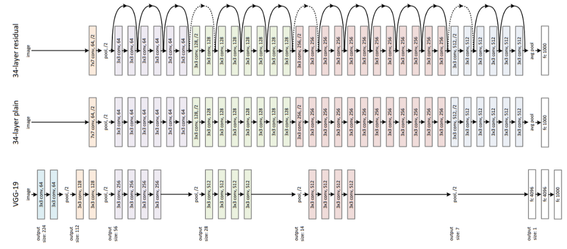
vgg19와 34-layer plain을 비교했을 때 34-layer는 가장 앞 layer에서 7x7 filter를 적용했고 레이어 수를 두 배 가까이 늘렸다
그리고 맨마지막에 flatten을 쓰지 않고 average pooling을 사용했더니 34-layer가 성능이 더 좋았다
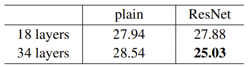
더 나아가 34-layer에서 residual block을 추가한 결과 추가하지 않은 것보다 오차율이 감소한 것을 확인할 수 있었다
Residual block과 Batch Normalization의 조합으로 훨씬 더 깊은 layer가 가능해졌다
결국 총 152 layer를 쌓을 수 있게 되었다
'Computer_Science > Visual Intelligence' 카테고리의 다른 글
| 22일차 - 논문 수업 (Learning Technique / numerical stability) (0) | 2021.10.15 |
|---|---|
| 21일차 - 논문 수업 (CNN / Data Augmentation) (0) | 2021.10.15 |
| 19일차 - 논문 수업 (CNN) (0) | 2021.10.08 |
| 18일차 - 논문 수업 (CNN) (0) | 2021.10.08 |
| 17일차 - 논문 수업 (CNN) (0) | 2021.10.04 |