728x90
반응형
import pandas as pd
drinks = pd.read_csv('drinks.csv')
drinks.info

<bound method DataFrame.info of          country  beer_servings  spirit_servings  wine_servings  \
0    Afghanistan              0                0              0
1        Albania             89              132             54
2        Algeria             25                0             14
3        Andorra            245              138            312
4         Angola            217               57             45
..           ...            ...              ...            ...
188    Venezuela            333              100              3
189      Vietnam            111                2              1
190        Yemen              6                0              0
191       Zambia             32               19              4
192     Zimbabwe             64               18              4

     total_litres_of_pure_alcohol continent
0                             0.0        AS
1                             4.9        EU
2                             0.7        AF
3                            12.4        EU
4                             5.9        AF
..                            ...       ...
188                           7.7        SA
189                           2.0        AS
190                           0.1        AS
191                           2.5        AF
192                           4.7        AF

[193 rows x 6 columns]>
drinks.head
<bound method NDFrame.head of country beer_servings spirit_servings wine_servings \
0 Afghanistan 0 0 0
1 Albania 89 132 54
2 Algeria 25 0 14
3 Andorra 245 138 312
4 Angola 217 57 45
.. ... ... ... ...
188 Venezuela 333 100 3
189 Vietnam 111 2 1
190 Yemen 6 0 0
191 Zambia 32 19 4
192 Zimbabwe 64 18 4
total_litres_of_pure_alcohol continent
0 0.0 AS
1 4.9 EU
2 0.7 AF
3 12.4 EU
4 5.9 AF
.. ... ...
188 7.7 SA
189 2.0 AS
190 0.1 AS
191 2.5 AF
192 4.7 AF
[193 rows x 6 columns]># 피처 상관관계
# 피어스 상관계수
# 'beer_serving', 'wine_servings'
corr = drinks[['beer_servings', 'wine_servings']].corr(method = 'pearson')
corr
beer_servings wine_servings
beer_servings 1.000000 0.527172
wine_servings 0.527172 1.000000corr = drinks[['beer_servings','spirit_servings', 'wine_servings','total_litres_of_pure_alcohol']].corr(method = 'pearson')
corr
beer_servings spirit_servings wine_servings total_litres_of_pure_alcohol
beer_servings 1.000000 0.458819 0.527172 0.835839
spirit_servings 0.458819 1.000000 0.194797 0.654968
wine_servings 0.527172 0.194797 1.000000 0.667598
total_litres_of_pure_alcohol 0.835839 0.654968 0.667598 1.000000# 상관계수 시각화
import matplotlib.pyplot as plt
import seaborn as sns
cols_view = ['beer','spirit', 'wine', 'alcohol']
sns.set(font_scale = 1.5)
hm = sns.heatmap(corr.values, cbar = True, annot = True, square=True,
fmt = '.2f', annot_kws = {'size':15},
yticklabels = cols_view, xticklabels = cols_view)
plt.show()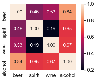
hm = sns.pairplot(drinks)
plt.show()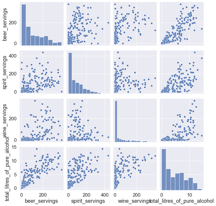
drinks.isnull().sum()
# drinks.info()

country                          0
beer_servings                    0
spirit_servings                  0
wine_servings                    0
total_litres_of_pure_alcohol     0
continent                       23
dtype: int64
drinks['continent'] = drinks['continent'].fillna('OT')
drinks['continent'].value_counts()
AF 53
EU 45
AS 44
OT 23
OC 16
SA 12
Name: continent, dtype: int64# 대륙별 국가수 출력
print(drinks.groupby('continent').count()['country'])
continent
AF 53
AS 44
EU 45
OC 16
OT 23
SA 12
Name: country, dtype: int64plt.pie(drinks['continent'].value_counts(),
labels = drinks['continent'].value_counts().index.tolist(),
autopct='%.0f%%',
explode = (0,0,0,0.2,0,0),
shadow=True)
plt.title('null data to "ot"')
plt.show()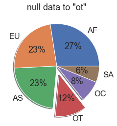
drinks.groupby('continent')['spirit_servings'].max()

continent
AF    152
AS    326
EU    373
OC    254
OT    438
SA    302
Name: spirit_servings, dtype: int64
drinks.groupby('continent')['spirit_servings'].mean()
continent
AF 16.339623
AS 60.840909
EU 132.555556
OC 58.437500
OT 165.739130
SA 114.750000
Name: spirit_servings, dtype: float64drinks.groupby('continent')['spirit_servings'].agg(['mean','min','max','sum'])
mean min max sum
continent
AF 16.339623 0 152 866
AS 60.840909 0 326 2677
EU 132.555556 0 373 5965
OC 58.437500 0 254 935
OT 165.739130 68 438 3812
SA 114.750000 25 302 1377dm = drinks['total_litres_of_pure_alcohol'].mean()
con_mean = drinks.groupby('continent')['total_litres_of_pure_alcohol'].mean()
con_mean[con_mean >= dm]
continent
EU 8.617778
OT 5.995652
SA 6.308333
Name: total_litres_of_pure_alcohol, dtype: float64dmax = drinks.groupby('continent')['beer_servings'].mean()
dmax[dmax == dmax.max()]
continent
EU 193.777778
Name: beer_servings, dtype: float64drinks.groupby('continent')['beer_servings'].mean().idxmax()
# 'EU'drinks.groupby('continent')['beer_servings'].mean().idxmin()
# 'AS'result
mean min max sum
continent
AF 16.339623 0 152 866
AS 60.840909 0 326 2677
EU 132.555556 0 373 5965
OC 58.437500 0 254 935
OT 165.739130 68 438 3812
SA 114.750000 25 302 1377result.index
# Index(['AF', 'AS', 'EU', 'OC', 'OT', 'SA'], dtype='object', name='continent')import numpy as np
# result = drinks.groupby('continent')['beer_servings'].agg(['mean', 'min', 'max', 'sum']
means = result['mean'].tolist()
mins = result['min'].tolist()
maxs = result['max'].tolist()
sums = result['sum'].tolist()
index = np.arange(len(result.index))
bar_width = 0.1
rects1 = plt.bar(index, means, bar_width, color = 'r', label = 'Mean')
rects2 = plt.bar(index, mins, bar_width, color = 'g', label = 'Min')
rects3 = plt.bar(index, maxs, bar_width, color = 'b', label = 'Max')
rects4 = plt.bar(index, sums, bar_width, color = 'y', label = 'Sum')
plt.xticks(index, result.index.tolist())
plt.legend(loc="best")
plt.show()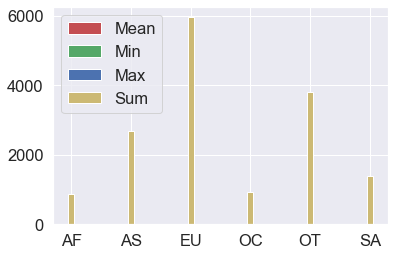
# 대륙별 total_litres_of_pure_alcohol 섭취량 평균을 시각화
import numpy as np
continent_mean = drinks.groupby('continent')['total_litres_of_pure_alcohol'].mean()
total_mean = drinks.total_litres_of_pure_alcohol.mean()

continents = continent_mean.index.tolist()
continents.append('Mean')

x_pos = np.arange(len(continents))
alcohol = continent_mean.tolist()
alcohol.append(total_mean)

bar_list = plt.bar(x_pos, alcohol, align = 'center', alpha = 0.5)
bar_list[len(continents)-1].set_color('r')
plt.plot([0., 6], [total_mean, total_mean], "k--")
plt.xticks(x_pos, continents)
plt.ylabel('total_litres_of_pure_alcohol')
plt.title('total_litres_of_pure_alcohol by continent')
plt.show()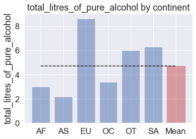
# 대륙별 beer_serving 합계를 막대그래프로 시각화
# eu 막대의 색상을 빨강색으로 변경하기
# 전체 맥주 소비량 합계의 평균을 구해서 막대 그래프에 추가
# 평균선을 출력하기, 막대 색상은 노랑색
# 평균 선은 검정색("k--")
beer_sum = drinks.groupby('continent')['beer_servings'].sum()
beer_sum

continent
AF    3258
AS    1630
EU    8720
OC    1435
OT    3345
SA    2101
Name: beer_servings, dtype: int64
beer_mean = beer_sum.mean()
beer_mean
# 3414.8333333333335continents = beer_sum.index.tolist()
continents.append("Mean")
continents
# ['AF', 'AS', 'EU', 'OC', 'OT', 'SA', 'Mean']x_pos = np.arange(len(continents))
alcohol = beer_sum.tolist()
alcohol.append(beer_mean)
alcohol
[3258, 1630, 8720, 1435, 3345, 2101, 3414.8333333333335]
bar_list = plt.bar(x_pos, alcohol, align='center', alpha = 0.5)
bar_list[2].set_color("r")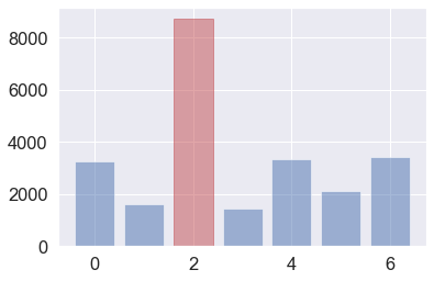
반응형
'Data_Science > Data_Analysis_Py' 카테고리의 다른 글
| 20. 서울시 인구분석 || 다중회귀 (0) | 2021.11.23 |
|---|---|
| 19. 세계음주데이터2 (0) | 2021.11.23 |
| 17. 서울 기온 분석 (0) | 2021.11.02 |
| 16. EDA, 멕시코식당 주문 CHIPOTLE (0) | 2021.10.28 |
| 15. 스크래핑 (0) | 2021.10.28 |